Note: This year I have decided not to lecture on the physical principles of cardiovascular measurements. Instead I would like to explore some of the mistakes and errors in cardiovascular medcal practice that have been made in the past and, in some cases, are still being made today. See last year's notes if you are interested in basic lectures in physical principles of measurement.
"Half of everything that we teach
to medical students is wrong...
The problem is that no one knows which half."
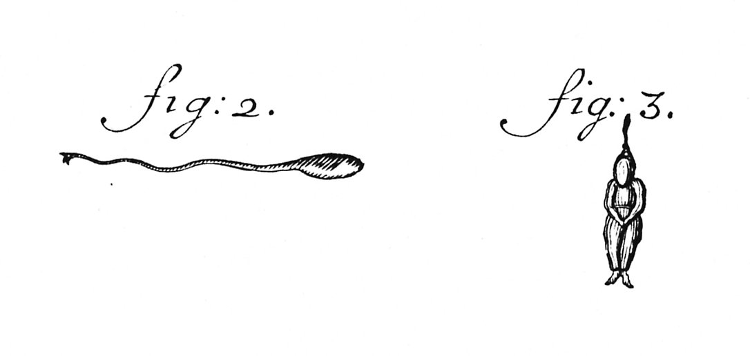
1. Scientists and doctors are human and seeing what we expect to see is a human trait. Perhaps the most obvious example of this is the sketch of human spermatozoa by Dalenpatius in the very early days of microscopy (fig: 3 below). We know about it today because of a letter by Leeuwenhoek (the inventor of the microscope) dated 1702 correcting Dalenpatius' observations (fig: 2).
Because of the diffraction limit inherent in microscopy, sperm are difficult to see, particularly in the early, hand-made microscopes using natural light. Because everyone knew that a sperm was a small version of a person (a homunculus), it seems that is what was seen.
2. We frequently don't use all of our rational facilities, particularly when we are confronted by something that 'looks' right. This fact is frequently exploited by advertisers. What is wrong with this plot?
A give away is the lack of any numbers on the pain axis. What are the units of pain? (A figure similar to this stimulated a contest amongst my fellow postgraduates for the best unit of pain - 'sacks of woe' was my favorite.)
The maximum rate of decrease of left ventricular pressure (max -dPLV/dt) is frequently used clinically as an index of diastolic function of the LV. It is affected both by the rate of myocarcial relaxation and by incoordination of the ventricle. Recently Prof. M. Sugawara of Tokyo Women's Medical College pointed out to me that virtually every text book on haemodynamics contains an error pertinant to this parameter. Here are a few examples - note the time at which (max -dPLV/dt) occurs relative to the dicrotic notch.
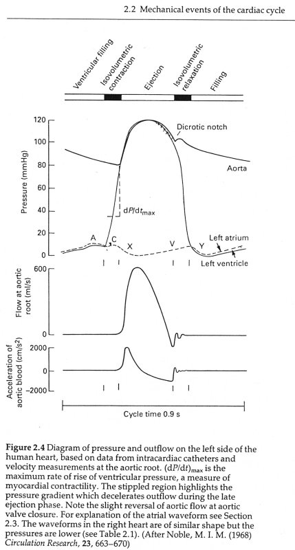
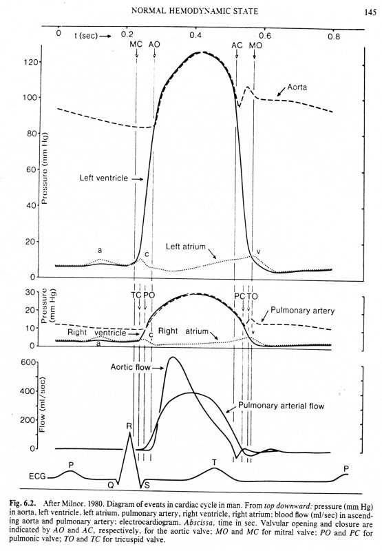
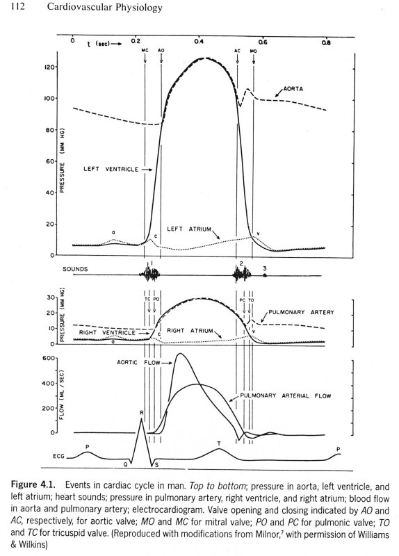
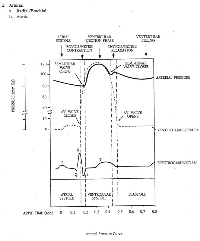
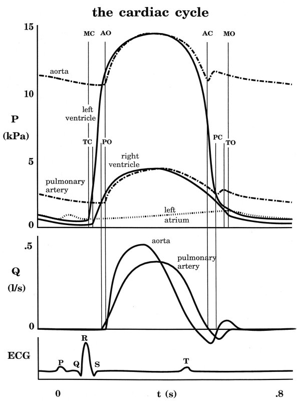
The first two sketches are from Milnor, the first from The Heart and the second from Hemodynamics, which came out later. The third is from the current edition of Levick, An Introduction to Cardiovascular Physiology, one of the standard medical textbooks on the subject. The fourth is from a tutorial on cardiac perfusion currently supplied by Datascope as a teaching aide for those using their intra-aortic, counter-pulsation balloon ventricular assist device. Just to prove that I am being dispassionate and honest, the last is from my lecture notes on cardiovascular mechanics used in last year's course. In every case, the rate of decrease of PLV continues to increase after the dicrotic notch, the time of aortic valve closure. This means that (max -dPLV/dt) occurs during the isovolumic relaxation phase of the cardiac cycle when both the aortic and mitral valves are closed.
Here is a typical example of a measurement of PLV and PAo taken in a dog under control conditions (measurements in man are very similar).
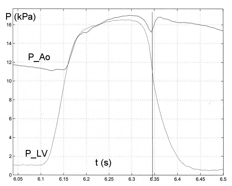
The vertical line in the figure indicates the time of (max -dPLV/dt), which occurs simultaneously with the dicrotic notch and hence the time of aortic valve closure. This has been true in every measurement that I have seen (since Prof. Sugawara pointed out the error to me) and I now believe that this is what happens normally.
There is a mechanical explanation why the rate of maximum negative dPLV/dt occurs before (or at) the time of closure of the aortic valve. The flow of blood in the aorta produced during systole has inertia and when the LV starts to relax this inertia influences the ventricle, causing a kind of suction. As long as the aortic valve is open, the pressure in the LV will be dictated by both the rate of relaxation of the myocardium and the suction effect of the blood flowing in the aorta. Since the aortic valve is passive and closed by the reversal of the direction of the flow in the ascending aorta, the closure of the aortic valve indicates the time when aortic velocity reverses and the suction effect ends. In any case, the closure of the valve would isolate the ventricle from what is happening in the aorta. It seems that the suction effect is important, because (max -dPLV/dt) occurs before (or at) the time of aortic valve closure. In fact, there is generally a distinct point of inflection in PLV at the time of the dicrotic notch with PLV falling more slowly during the period of the isovolumetric relaxation phase.
This is not simply of academic interest. If it is assumed that (max -dPLV/dt) occurs during the isovolumic relaxation phase it would be independent of the pattern of aortic blood flow and hence the previous systolic phase of the cycle. If, however, it is dependent upon both the rate of myocardial relaxation and the blood flow resulting from systole, then its value as a clinical indicator of diastolic function is suspect.
"The authors should know that the
cardiovascular system
is in a state of steady state oscillation."
This quote comes from a referee's comment about one of our recent (as yet unpublished) papers on arterial mechanics. It expresses a very commonly held belief about the cardiovascular system. Is it true?
An intriguing argument against steady state oscillation has been advanced by Prof. JV Tyberg of Calgary. He notes that diving mammals decrease their heart rate significantly when they dive - e.g. the Wardell seal decreases its surface heart rate by a factor of 7 when it dives. Since the wavelength of an oscillatory wave is given by the wave speed divided by the frequency, this means that if the wave speed in the arteries remains roughly constant, a reasonable assumption since the wave speed is determined by the distensibility of the arteries which cannot change too much, the wavelength in the diving Wardell seal would have to increase by a factor of approximately 7. This would be difficult because the anatomy of the seal does not change when it dives.
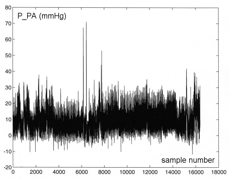
The most persuasive evidence against steady-state oscillation, in my opinion, is what happens during ectopic beats. The 'missing' beats occur spontaneously in most normal circulations but are more frequent in the stressed or diseased circulation. The following figure shows the pressure in the main pulmonary artery in the dog during a period of hypoxia.
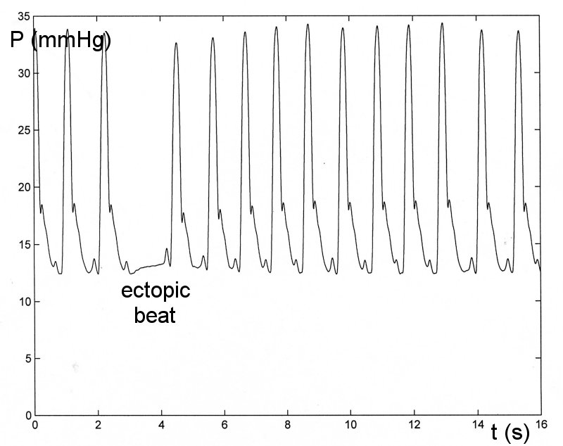
We see that when the heart is beating regularly the pressure does look very regular, just as it would if the pulmonary circulation was in steady-state oscillation. However, when the heart does not beat, the ectopic beat, there is no hint of an oscillation in pressure. This is not the behaviour of a system in steady-state oscillation. For eample, a playground swing is kept in steady-state oscillation in the presence of friction and air resistance by appropriately timed pushes. If one of the pushes is missed, the swing still swings during the 'missed' beat, just not as far as normal. The rapid cessation of the motion seen during the ectopic beat is characteristic of an 'over-damped' system. By their nature, over-damped systems cannot exhibit steady-state oscillation.
A final, less convincing, argument against steady-state oscillation is that they are usually the result of some 'tuning' of the system. Since the circulatory system operates over a wide range of frequencies, heart rates can easily double during excercise, it would be hard to obtain the necessary tuning under all conditions. An interesting suggestion for oscillatory behaviour, is the speculation that top class marathon runners could adjust their stride to coincide with their heart rate so that the forces on the arteries and veins caused by the heel strike could be transforme into increased performance during races.
Kilner, et al. [get reference to Nature paper, 2000 or 2001] have suggested that the shape of the mammalian heart may have evolved so that the direction of influx and efflux are opposite to each other, unlike the hearts of more primative species where the blood flows in the same direction into and out of the heart. They argue that there could be some natural resonance in the design that makes the process more efficient by using the momentum of the flowing blood.
First of all, the normal circulation normally looks very regular, as if it was in steady-state oscillation. It is only during perturbations such as ectopic beats that the regularity is lost.
Secondly, and more subtly, I suspect that it may have something to do with the success of Fourier analysis.
Fourier's theorem states that any periodic function can be represented exactly by an infinite series of sines and cosines with frequencies that are integer multiples (harmonics) of the fundamental frequency. He also derived the inverse of the transform so that the inverse transform of the transformed function is exactly the original function. With the advent of the fast Fourier transform this method of analysis has been used very extensively in cardiovascular studies. It has become so common that the standard textbooks on haemodynamics [get references] start their chapters on arterial mechanics by introducing the Fourier transform.
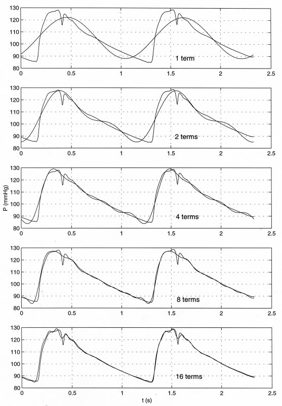
The the data are the pressure in the ascending aorta measured in man during routine catheterisation and the panels show the representation of the data by an increasing number of terms in the Fourier transform. The top panel shows the fit due to the fundamental term; the second the fit with the fundamental and the first harmonic; the middle panel the fit with the fundamental and the first 3 harmonics (4 terms); the fourth panes the fit with 8 terms and the lower panel the fit with 16 terms. The utility of the method is evidenced by the excellent fit to the data obtained with only sixteen terms in the Fourier series transform of the measured data.
Another example is the Fourier analysis of the data shown above for the pressure in the main pulmonary artery with the ectopic beat.
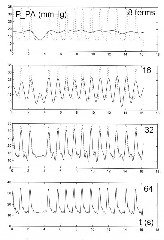
In this figre the dotted line is the measured data and the solid line is the fit using progressively more terms in the Fourier transform. For this example with more cycles to be fit over the time of the measurement it is necessary to use more terms to adequately describe the data. However, even for this case only the first 64 terms of the Fourier transform are needed to obtain a very good approximation to the measured data.
The success of the Fourier transform in describing the measured cardiovascular data might appear to be an argument that it is an oscillatory process. However, this is not true. Since Fouier's theorem mathematicians have shown similar transforms can be defined using any set of complete, orthogonal functions. The following are some examples of complete, orhogonal functions that can be used to define an exact transformation of any function or measurment.
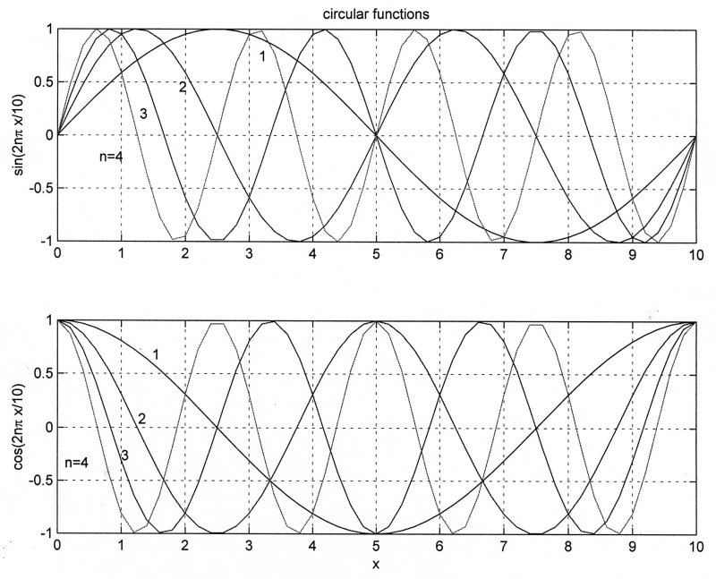
These are the circular functions, better known as sines and cosines, which were used by Fourier.
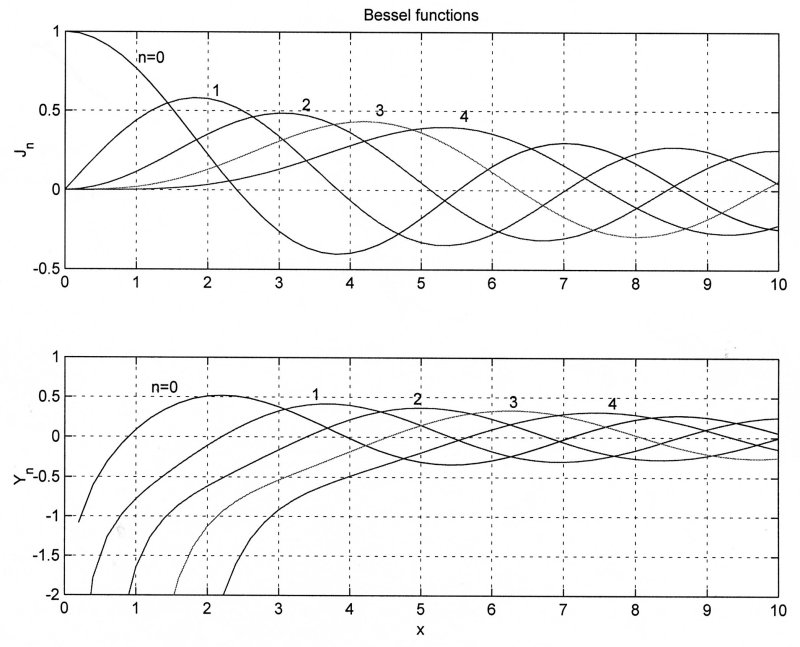
These are Bessel functions of the first and second kind which were used by Hankel to define the Hankel transformation. It is very useful for problems involving axisymmetry.
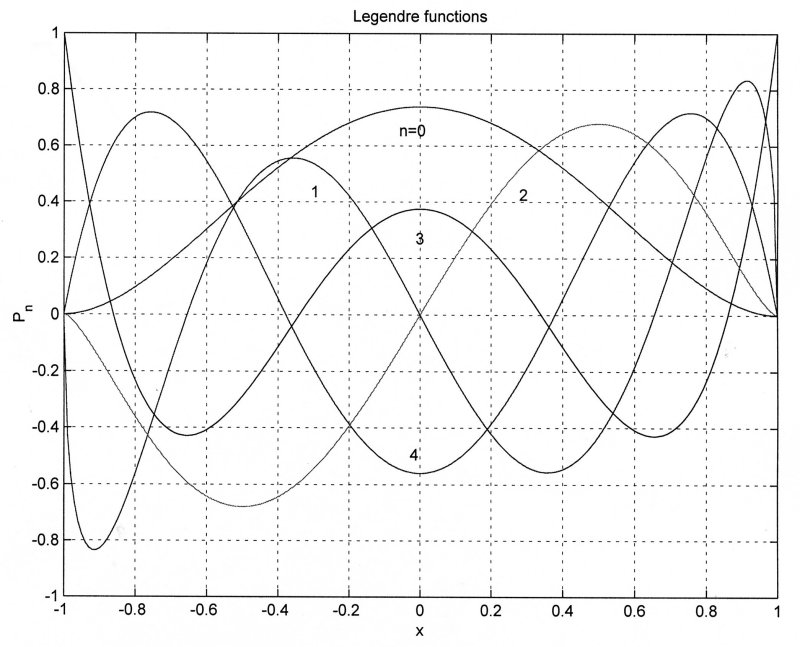
These are Legendre functions defined using polynomials. Because of the simplicity of their definition, they are very commonly used in numerical analysis.
It has been shown that there are an infinity of complete, orthogonal functions that could be used to define exact transformations. Thus, the use of the periodic circular functions to describe cardiovascular data is only one of an infinite number of possibilities and cannot be used to deduce that the cardiovascular system is in steady state oscillation.
Things were made even more confusing about a decade ago when another type of transformation was discovered, the wavelet transformation. At first it was simply an approximate method, but Daubechies [get reference] discovered a whole new class of 'orthogonal' wavelets that could be used to define a complete transformation of any function or measured data together with an inverse function that could be used to recover the original data exactly. Since her original discovery, many other examples of orthogonal wavelets have been discovered. Four of them are illustrated in the following figure.
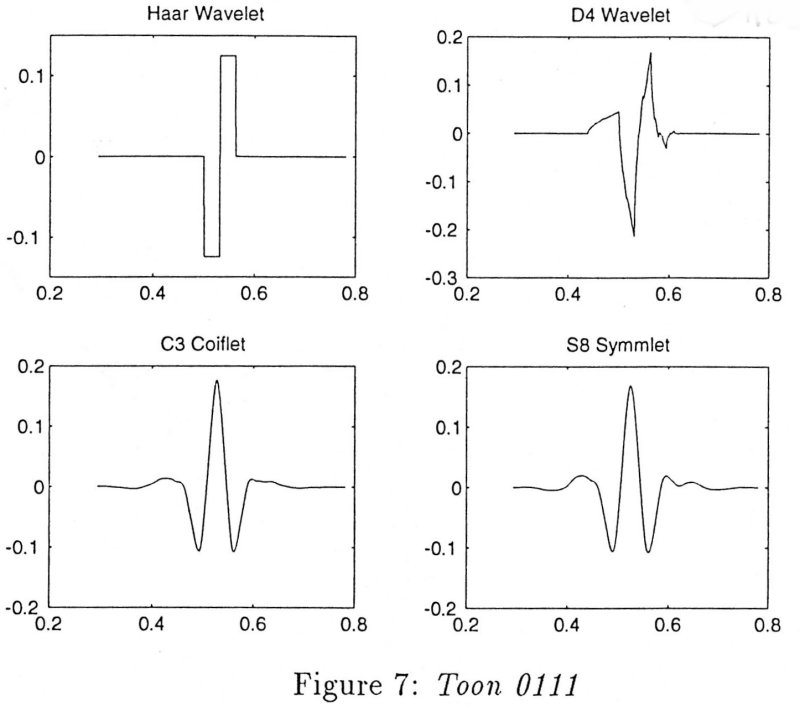
The wavelet labelled D4 is one of the orthogonal wavelets defined by Daubechies, note that it is rather irregular and not obviously representative of any particular physical process. It is not even continuously differentiable. The Coiflet orthogonal waveform is the one that is used in the example below. A few years ago, it was discovered that there are an infinity of orthogonal wavelets that can be used to completely transform any function or measured data. The ability of the periodic circular functions to model cardiovascular data is now doubly-infinitely non-unique.
The algorithm used to obtain the wavelet transform is fairly straightforward in principle. The wavelet function is scaled to the full period of the data and the multiplicative coefficient that gives the best fit of the wavelet function to the whole of the data using a least squares fit. The data is divided into two halves, the wavelet is scaled to half of the total period and a coefficient is determined for each half. The data is then divided into four quarters, the wavelet is scaled to one quarter of the total period and 4 best fit coefficients are determined. The halving of the fitting interval is continued indefinitely for analytical functions or until there is only one point per division for discrete data. The coefficients thus determined comprise the wavelet transformation of the original function (the inverse of the transform is a little more difficult to define simply).
One of the reasons for using wavelet transforms is the non-stationary nature of most medical or physiological data. For example, Dr. JSR Gibbs measured the pressure in the main pulmonary artery of mountaineers who suffered from high altitude pulmonary oedema (HAPE) and were studied for 3 days continuously while in an altitude chamber where the pressure was varied to mimic a trip to altitude. The data for one day illustrate the highly non-stationary nature of the data.
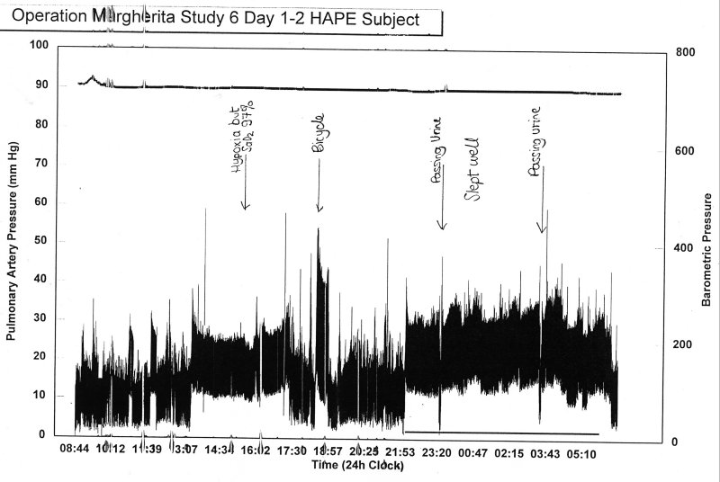
The pulmonary pressure varies significantly with posture, wakefulness, exercise, urination, etc., and so it would be advantageous to find a method of analysis that did not presume strict periodicity of the data being transformed. As an example we have taken a 512 s section of the data to analyse (since the data were sampled 32 times a second, this corresponds to 16348 points).
The wavelet transform using the Coiflet orthogonal wavelet is represented graphically in the following figure where the numbers on the right refer to the power of 2 used to subdivide the total period of the data (2-1 = 1/2, 2-2 = 1/4, ... 2-14 = 1/16348). The bars represent the best fit coefficient of the suitably scaled wavelet to the data over the interval around the bar.
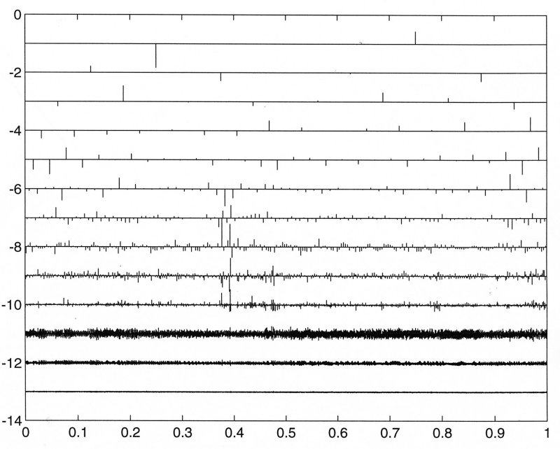
To get a better idea of the meaning of the transform, the coefficients are multiplied by the scaled wavelets to obtain a continuous signal at each scale of subdivision which represents the best fit to the data at the corresponding period. While this is not strictly a frequency, it is conceptually equivalent and gives some insight into the interpretation of the transform.
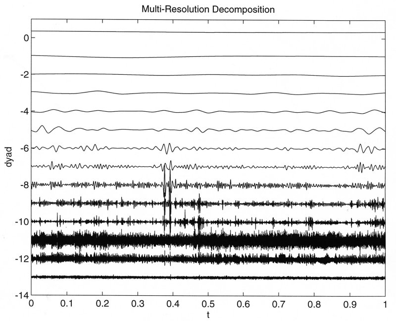
The most useful feature of the wavlet transform compared to integral transforms based on complete, orthogonal functions is that the time axis is retained. This means that it is possible to relate particular features of the wavelet spectrum to temporal events in the data. In the above example we see that the two very large spikes in pulmonary pressure occuring at about 6000 sample points are reflected in the wavelet spectrum by very large amplitude coefficients at the scaled time 0.4. This enables us to use the temporal information in the original data to help us interpret the wavelet transform of the the data.