This lecture will deal not with a systematic exposition of cardiovascular measurement techniques but with some problems and errors that have arisen or are current in cardiology. It is hoped that some of the techniques used will be made clearer in this way.
Some specific problems in ultrasound measurements in the heart:
1) Resolution
The wavelength of an ultrasound wave depends upon the frequency produced by the transducer and the speed of sound in the tissue. Because higher frequency sound waves dissipate more quickly due to viscous and viscoelastic effects, the maximum frequency is limited by the distance to the target. For transthoracic scans, the maximum frequency is generally 3.5 MHz. For transoesophogeal scans the distance to the heart is smaller and 5 MHz transducers are commonly used.
wavelength = (speed of sound)/frequency
The speed of sound in tissue is approximately 1500 m/s (the speed of sound in water). Therefore, for a 5 MHz transducer the
wavelength = (1500)/(2p 5x10⁶) ~ 50 mm
The absolute, ideal resolution attainable is 1/2 a wavelength and so the ultimate resolution for a 5 MHz probe is > 25 mm.
This means that it is impossible to make accurate measurements of features such as heart valve thicknesses or the intimal thickness of blood vessels, despite the claims of some researchers.
2) Diffraction
Different tissues have different wavespeeds which means that as the beam traverses different tissues it will be diffracted. (The fish in the aquarium is not where it appears to be for the same reason.) In an abdominal scan, it is estimated that the difference between apparent and actual position can be as much as 3 cm. How is it possible to do lumbar punctures under ultrasonic guidance?
3) Systolic Anterior Motion (SAM) in hypertrophic cardiomyopathy
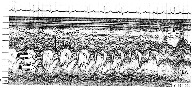
SAM is the acronym for systolic anterior movement of the anterior leaflet of the mitral valve during systole, a time when the leaflet should be movin posteriorly. In extreme cases this can lead to obstruction of the left ventricular outflow tract by the anterior leaflet and when it is observed in patients with hypertrophic cardiomyopathy it is often taken as an indication for intervention. The short axis view of the left ventricle is obtained from an intercostal view.
![]()
(from H. Feigenbaum, Echocardiography, 4th Ed.)
The beam marked 2 in the figure passes through both mitral valve leaflets and this view can be used to observe their motion during the cardiac cycle.
(adapted from H. Feigenbaum, Echocardiography, 4th Ed.)
Because the whole heart is moving, it is not anterior motion relative to the transducer, but anterior motion relative to the endocardium that should be measured. In this text book example, note the movement of the valve leaflet (top arrow) and the simultaneous movement of the posterior left ventricular wall (bottom arrow). This is often overlooked in cardiac scans.
4) Filling of the left ventricle (LV)
It is relatively easy to measure the velocity of blood flow through the mitral valve using range gated Doppler ultrasound.
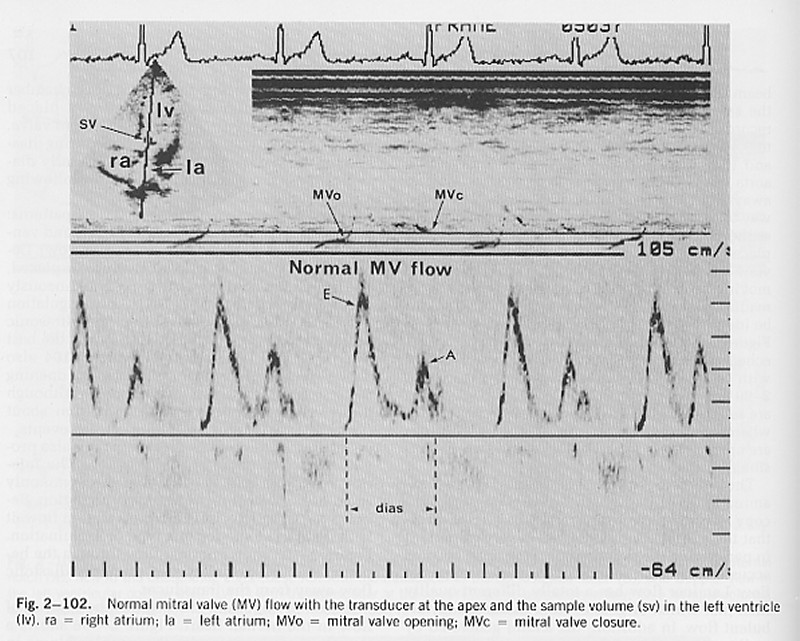
(from H. Feigenbaum, Echocardiography, 4th Ed.)
In the normal heart at rest, two separate periods of blood flow through the mitral valve are seen: the 'E wave' which occurs soon after closure of the aortic valve and the 'A wave' which is the result of atrial contraction (note the timing of the A wave relative to the P wave on the ECG). It is often assumed that the net flow into the ventricle can be calculated by integrating the measured velocity times the area of the mitral valve ring. This is wrong!
The velocity is the velocity relative to the transducer which is fixed to the chest wall. As the atrium contracts, the mitral valve moves towards the apex. Thus, blood which is initially in the atrium can find itself in the ventricle not because it has moved relative to the transducer, but because the left ventricle has moved.
This is similar to the mechanism of the old fashioned hand operated pump. In the well is a cylinder with a hinged plate at the bottom. As the handle is raised, the cylinder descends into the well water and the hinged plate swings open admitting water into the cylinder. When the handle is lowered, the cylinder moves upward, the hinged plate closes and the water is elevated. The cylinder is filled by moving it relative to the water in the well which is stationary relative to the surface.
A note in passing: By using the ECG as a temporal reference, it is possible to compare the timing of different events measured from different views and by different methods during the cardiac cycle. One common observation that, as yet is completely unexplained mechanicially, is the opening of the mitral valve leaflets well before there is any flow through the valve orifice. This is a research project crying out to be done.
The Doppler principle can be used to measure the velocity of movement of tissue in the direction of the ultrasound beam. Because the velocities are generally much lower than that of blood, the frequency shift is correspondingly lower and more difficult to measure. Modern ultrasound machines, however, frequently offer 'tissue Doppler' as an option and it is being used with increasing frequency in echocardiology.
A common use is to assess the long axis function of the left ventricle. Using M-mode from the apical view, it has long been possible to measure the movement of the mitral ring.
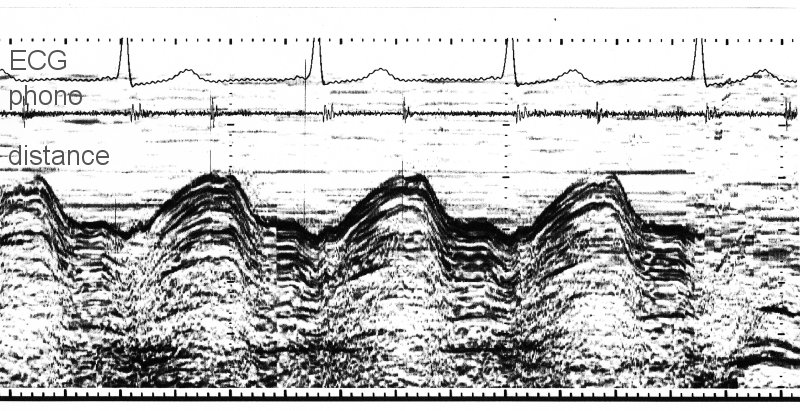
Using the ECG as a temporal reference, it can be seen that the mitral ring moves upwards (towards the apex) during systole and downwards (away from the apex) during diastole. In this patient, the filling in early diastole (the E wave of mitral filling) causes a very rapid increase in the long axis. There is also a small increase associated with the contraction of the atrium (the A wave).
The tissue Doppler signal for the same patient was obtained from the same apical view by positioning the Doppler gate in the tissue adjacent to the mitral valve ring.
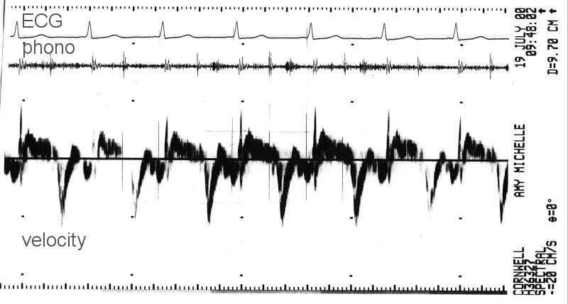
Shortening of the long axis was taken as positive velocity and so the large negative peaks of velocity correspond to the rapid increase in the long axis during the A wave of mitral inflow. Both representations of the motion of the mitral valve ring are valid and potentially useful.
The problem comes when it is assumed that the velocity signal is the derivative of the length of the long axis as measured from the M-mode signal. The long axis is measured at the interface between the blood and the mitral valve ring (the boundary in the M-mode signal). The tissue Doppler velocity is measured in a sample volume in the valve ring which, because of the movement of the heart relative to the ultrasound transducer, does not correspond to the same bit of tissue throughout the cycle. Therefore, what is being measured is not the velocity of the boundary of the ventricle, but the velocity of whatever tissue is within the sample volume at any particular time. The difference between the two can be significant since the motion of the heart within the chest cavity is comparable to the motion of the tissue relative to some fiducial point such as the centre of gravity of the heart.
6) The Modified Bernoulli Equation
Virtually every text book on echocardiography cites the modified Bernoulli equation for calculating the pressure difference (usually incorrectly called the 'pressure gradient') between two chambers of the heart when it is possible to measure the velocity of a jet between them using Dopple ultrasound. (Most heart valves permit a little bit of 'functional' regurgitation.)
DP = 4 V2
where (the better books add) P is measured in mmHg and V is measured in m/s2.
Think about the meaning of this equation in terms of dimensions.
The 'proper' Bernoulli equation is an energy equation for steady, non-dissipative flows. It says that along a stream line the total pressure, defined as the sum of the hydrostatic pressure (the potential energy) and the dynamic pressure (the kinetic energy) is constant.
P + 1/2rV2 = PTot
If we consider two points along the stream line: 1) in a region with a large cross section and hence low velocity (say the LV) and 2) in a high velocity jet (say a jet of mitral regurgitation).
P1 + 1/2rV12 = P2 + 1/2rV22 = PTot
If V1 ~ 0, then this equation can be rearranged to give DP = P1- P2 (writing V = V2)
DP = 1/2rV2
The density of blood is approximately 1050 kg/m3, and a pressure of 1 mmHg = 133.3 Pa. Substituting this into the Bernoulli equation
DP (mmHg) = 1/21050/133.3 V2 = 3.98 V2
The modified Bernoulli equation is simply using the fact that the density of blood measured in units of mmHg s2/m2 is approximately 8. That is, the '4' in the modified Bernoulli equation has dimensions. Should this sort of thing be encouraged?
7) Proximal Isovelocity Surface Area (PISA) measurement of volume flow rate
Jet velocities (U) are very easy to measure by Doppler ultrasound but jet areas (A) are very difficult to measure accurately. As a result, it is difficult to measure the volume flow rate (Q=UA) in a jet accurately.
PISA is a recent idea to get around this problem by looking not at the jet but the flow in the chamber where the jet is formed. It is based on the ideal solution for inviscid, steady flow in a semi-infinite reservoir flowing through a small hole at the origin (flow into a sink). Using a spherical coordinate system, it can be shown that the velocity is directed toward the origin with a magnitude (U) that depends only on the radius (R). For a steady flow, the volume flow rate across any hemiphere upstream of the jet must equal the volume flow rate in the jet.
Q = 2p R2 U
The suggested procedure is to find a region where the flow is hemispherical. Set the colour scale to give a particular colour at a convenient velocity (say 10 cm/s). Measure the radius where that velocity occurs and use the equation to calculate volume flow rate. Simple?
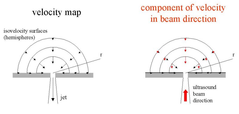
There is a fundamental error in this measurement. The Doppler probe measures not velocity but the component of velocity in the direction of the beam. Thus, if a sink flow was measured by Doppler on each isovelocity hemisphere, the component of velocity in the direction of the beam would vary with position on the hemisphere. Thus the Doppler velocity at the top of the hemisphere would be the isovelocity velocity but at all other points on the hemisphere the Doppler velocity would be reduced by the cosine of the angle of that point from the vertical. Near the plane, for example, the flow would be directed inward toward the origin (the location of the sink) and its component in the direction of the ultrasound beam would be very small.
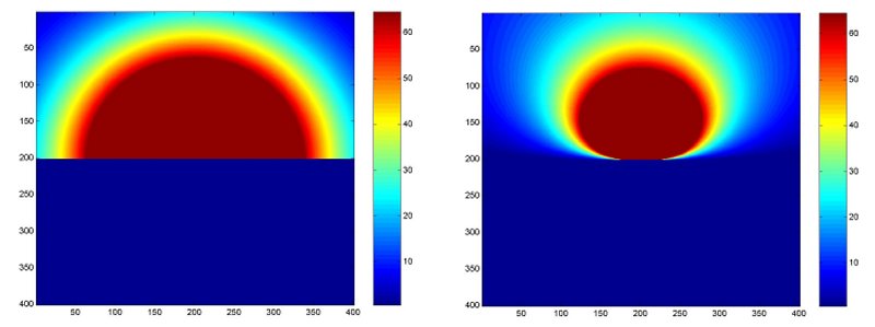
An idealised black and white version of what cardiologists look for when applying the PISA method together with what they should be looking for. As pointed out in the lecture, the method would still be valid if the pattern on the right was observed and the radius of the isovelocity hemisphere was taken from the radius of the new pattern directly over the origin of the jet.
In the assessment of valve stenosis, it would be very helpful to be able to measure the area of the stenosed valve. However, this is very difficult to do directly. Gorlin and Gorlin (1951) [get the reference] suggested an empirical way to determine the area of a stenosed valve using quantities that are more accesible to measurement. In a series of papers they developed equations for use with both the mitral and aortic valves. This equation is now in common use in cardiology. This is an example taken from the web-based program Medicalc
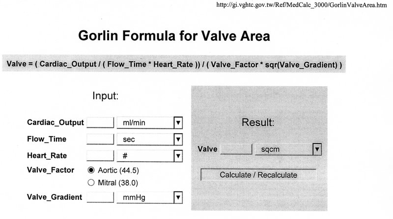
In symbols, this can be written
AV = CO/(TV HR K DP1/2)
where
| AV = area of the stenosed valve CO = cardiac output TV = time of flow through the valve HR = heart rate K = the Gorlin "constant" DP = the pressure difference across the valve |
What is the fluid mechanical basis of this equation?
First of all, it is useful to put the equation in terms variables that are more common in fluid mechanics. Since the total volume flow through through the valve must equal the cardiac output (what goes in must equal what goes out, on average), the volume passing through the valve per beat must be CO/HR. If the flow is steady, then the volume flow rate will be Q = CO/(HR TV). Finally, recall that the volume flow rate is the product of the velocity of the fluid times its cross sectional area, Q = VAV. Thus, we can see that this equation involves the pressure difference and the velocity - just like our old friend the Bernoulli equation.
The conservation of energy in the absence of viscous losses in a fluid is expressed by the Bernoulli equation
P1 + 1/2rV12 = P2 + 1/2rV22 = PTot
where PTot is a constant. If '1' is a reservoir where the velocity will be very small compared to the velocity through the jet, then we can rewrite it as
V2 = (2DP/r)1/2
or, in terms of the volume flow rate
Q = AVV2 = AV(2DP/r)1/2
For real orifice flows, there are two non-idealities that have to be considered. The first is the vena contracta, a jet flowing through an orifice of area A will contract to a smaller area. The area of contraction will depend on the exact design of the orifice and is usually denoted by the constant CC
A = CC AV
Second, real flows are viscous and there are always some viscous losses involved when flow passes through an orifice. Again, the losses are represented by a valve constant which relates the observed velocity to the ideal velocity corresponding to the measured pressure difference
V2 = CV (2DP/r)1/2
Combining both phenomena we can write
Q = CC CV AV(2DP/r)1/2
The coefficients measured for different sorts of orifices are shown in the following table taken from Streeter, Introduction to Fluid Mechanics [get reference]
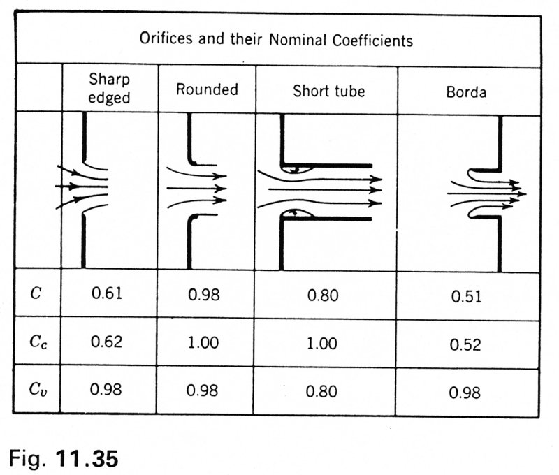
As a further complication, the orifice coefficient, C = CC CV, depends upon the Reynolds number of the flow through the orifice
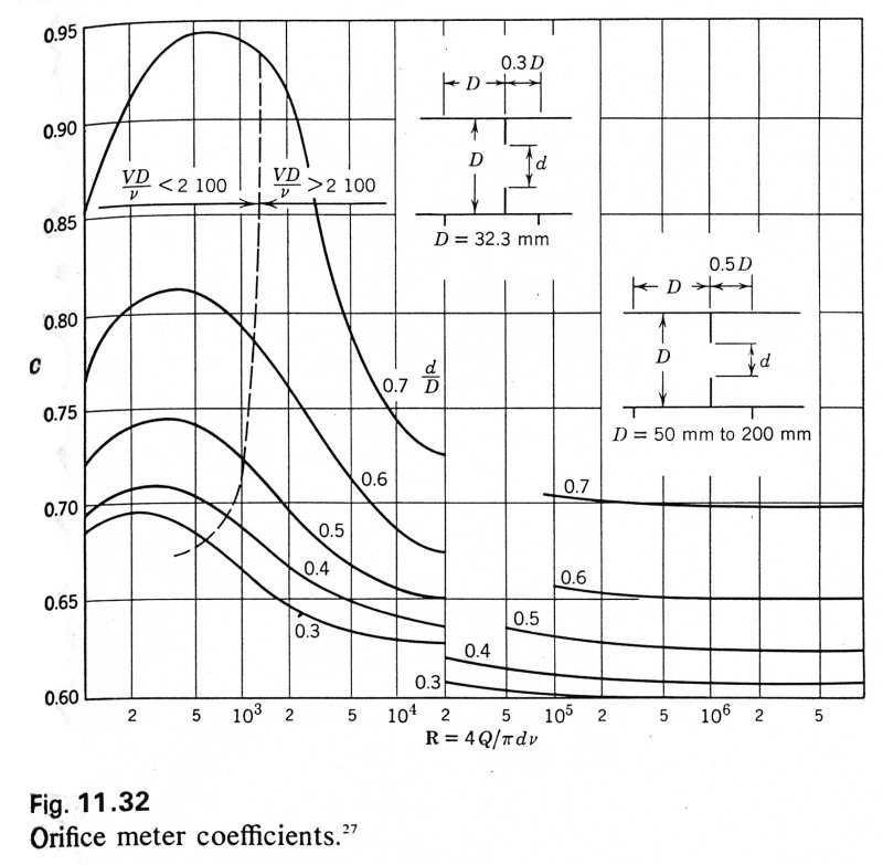
Comparing the two equations, we see that the Gorlin equation is equivalent to the orifice equation used by hydraulics engineers if
K = CC CV (2/r)1/2
With this derivation, it is clear why the Gorlin 'constant' is not really a constant, but is dependent upon the flow rate.
Allometric scaling is a type of 'scaling' analysis that is used commonly in some areas of physiology. It assumes that there is a power relationship between two variables
Y = a Xb
(Note that for this equation to have dimensionally integrity the constant a has to have the dimensions [Y]/[X]b). The values of a and b are most easily determined by plotting the data on a log-log plot
log Y = log a + b log X
where the slope is b and the intercept a. Here is an example of the metabolic rate (kcal/hr) as a function of body mass (kg) for species from unicellular organisms to mammals
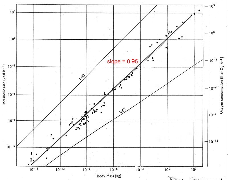
Note the extent of the abscissa, running from 10-15 to 10+3 kg (18 orders of magnitude). Fitting a best fit line through all of the points yields a line with slope = 0.95 which implies that metabolic rate varies almost with body mass. In fact, this is an example of one of the dangers of this type of analysis. The data as published is divided into three categories, unicellular organisms, poikilotherms and homeotherms.
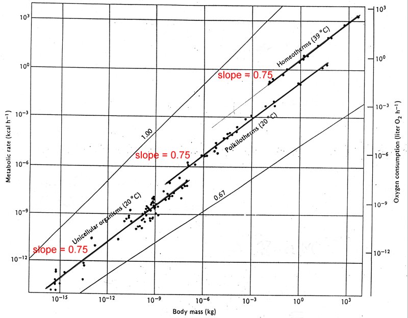
If we fit lines to each of these categories individually, we see that the slopes are all about 0.75, implying that the metabolic rate varies with body mass to the power of 3/4. With such large scales it is very easy to make errors of this magnitude. Note for example that the difference between the data and the fitted line for the smaller organisms is more than an order of magnitude.
If this analysis is applied to data for heart rate, HR, as a function of body mass, M, for mammals it is found that HR ~ M-0.25. That is, the smaller the mammal, the faster its heart rate. Applying it to the average life span, T, for the mammals, it is found that T ~ M+0.25. Since the total number of heart beats in a life time, N, is equal to the product of heart rate and life span, this implies that N is independent of body mass and so all mammals have a constant number of heart beats in a life time.
As it stands, this is a passingly interesting result about mammals on average. The danger comes when the result is expressed as 'the number of heart beats in a lifetime is invariant' and thus anything that reduces the heart rate will increase longevity. This is a fallacious and potentially a very dangerous argument. Carried to extreme, this would say that stopping the heart would lead to immortality.
Note: As pointed out in the lecture, the same argument applied to the scaling law for lifetime as a function of body mass would imply that one could increase one's lifetime by gaining weight!