"...for I dreamt last night of
bloody turbulence."
Troilus and Cressida - William Shakespeare
We will concentrate primarily on the interpretation of measurements of pressure and flow (or velocity) in the large arteries rather than the measurements themselves. Since about 50% of the population of the UK will die of arterial disease, a great deal of attention has been paid to the arteries. By comparison, relatively little is known about flow in veins
Pressure and flow in the large arteries exhibit complex, pulsatile waveforms
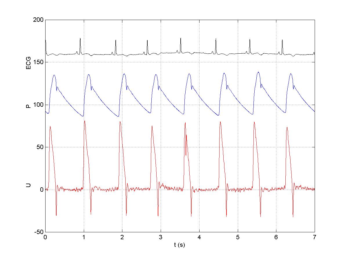
The figure shows the ECG (for reference), the pressure (P) in mmHg and the velocity (U) in cm/s in the ascending aorta. These data were measured invasively using a catheter.
One of the prominent features of arterial flow is that the pressure and velocity produced by the contraction of the left ventricle (LV) produce a wave which propagates throughout the arterial system, the pulse wave. These waves were first analysed scientifically by Thomas Young in his Croonian Lecture to the Royal Society in 1808.
Note that the flow is very pulsatile, increasing rapidly, reaching a peak, decelerating until the reversal of flow through the aortic valve closes the valves at the end of systole. There is no velocity during most of diastole. This is not true of flow in the carotid artery (and the uterine artery in pregnancy) where the flow is still pulsatile but there is substantial forward flow during the whole of diastole. Why do you think this is?
The 'stroke' volume ejected by the LV (approximately 50 ml) is slightly less than the volume of the ascending aorta. Therefore, the blood reaching the microcirculation is several heart beats 'away' from the LV.
Note that the pattern of flow in the coronary arteries is very different. Because the contraction of the myocardium occludes the vessels within it, flow during systole is either zero or greatly reduced. When the myocardium relaxes, blood can once again flow through the coronary microcirculation and so flow in the coronary arteries is highest during diastole. It has been argued that the need to perfuse the heart during diastole is the reason that the mean blood pressure in the systemic circulation is high. It has to drive flow through the coronary circulation during diastole.
Impedance Analysis
The standard way of analysing pressure and flow in the arteries is a Fourier transform based method generally known as impedance analysis in reference to the analogous analysis of electrical circuits.
Refer to:
Nichols and O'Rourke, MacDonald's Blood Flow in the Arteries (4th ed.).
Milnor, Hemodynamics.
In this method, the pressure, P(t), and velocity, U(t) (or, alternatively, the volume flow rate), are expressed as the linear superposition of sinusoidal waveforms using the Fourier transform
P(w) = F{P(t)}
U(w) = F{U(t)}
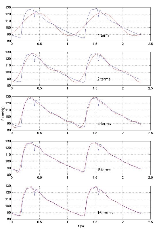
Surprisingly few harmonics are necessary to build up a very good approximation to the experiementally measured waveforms. This is shown here where the original waveform (in blue) is compared to the first harmonic wave (in red), the sum of the first and second harmonics, the sum of the first four harmonics, eight harmonics and finally sixteen harmonics. We see that sixteen harmonics are sufficient to reproduce most of the detail of the measured waveform.
Because the Fourier transform is complete, summing all of the harmonics will give the initial waveform exactly, noise and all.
By analogy to Ohms law, relating voltage and current in electrical circuits, it is assumed that the pressure and velocity for each harmonic are related
P(w) = U(w) Z(w)
where Z(w) is called the impedance. Because P(w) and U(w) are complex numbers (they have a real and imaginary part), Z(w) is also complex. It is usually represented by the polar form, i.e. its magnitude |Z| and phase f, where
Z(w) = |Z| eif
For the data shown previously, the second beat in the figure showing P and U above,
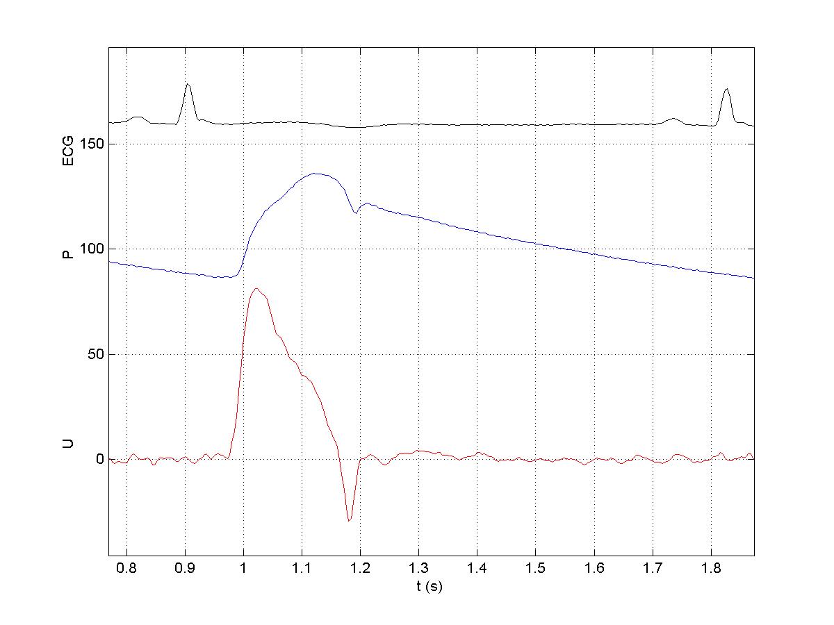
the P(w) and U(w), magnitude and phase, are

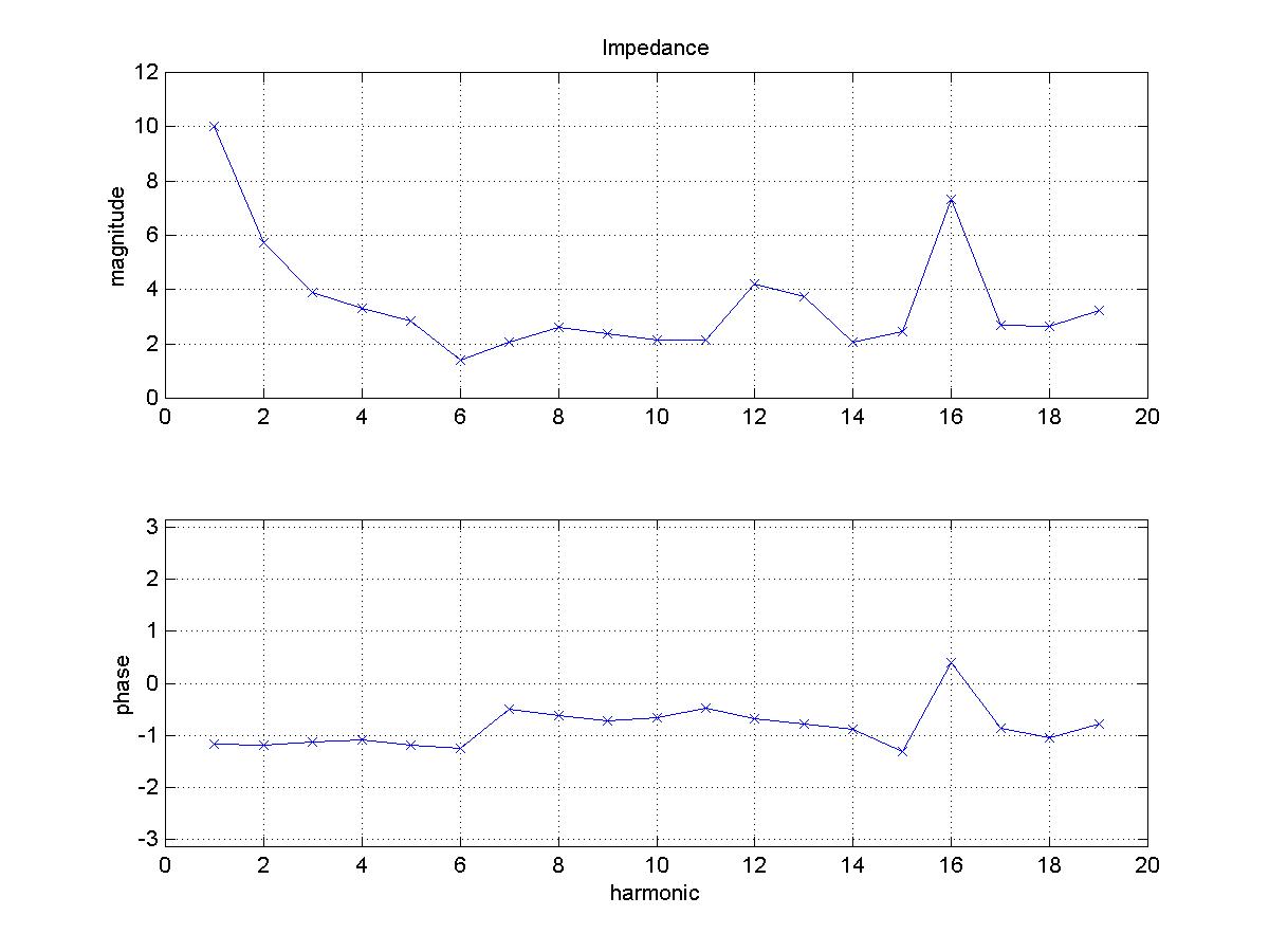
The impedance, magnitude and phase, calculated from these data is
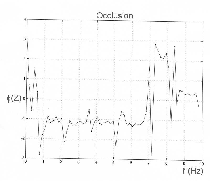
As an example of impedance analysis, we apply it to data which were recorded during an experiment on the effect of aortic occlusion of pressure and flow in the ascending aorta. The control conditions are shown on the left and the data recorded during total occlusion of the upper thoracic aorta are shown to the right. The measured data are
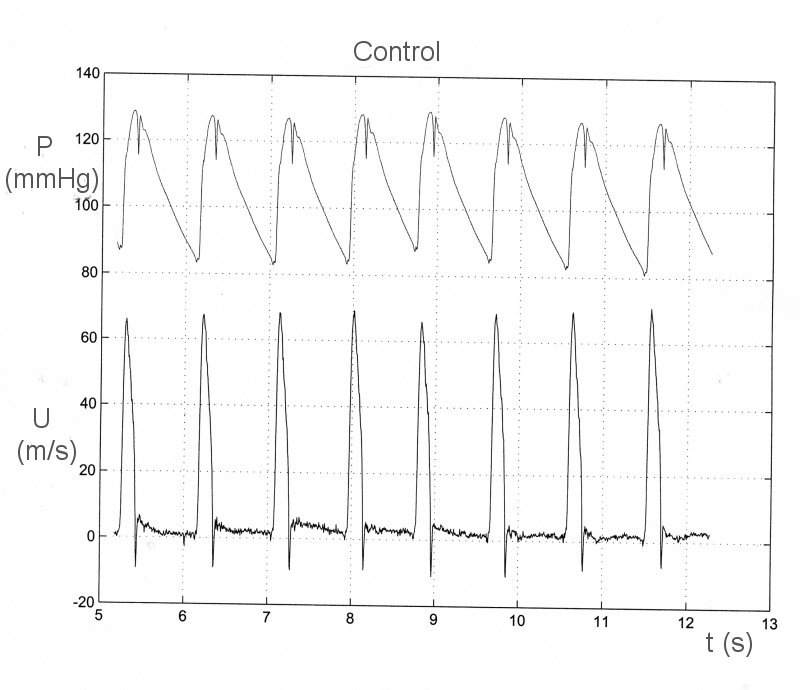
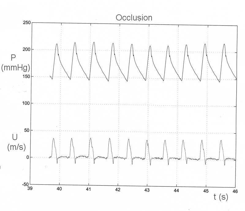
The Fourier transforms of P and U are complex. The magnitudes are
![]()
![]()
The phases are

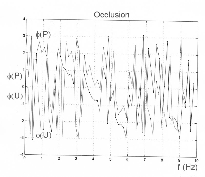
The impedance is calculated at each frequency as Z = P/U. They too are complex numbers. The magnitudes are
![]()
![]()
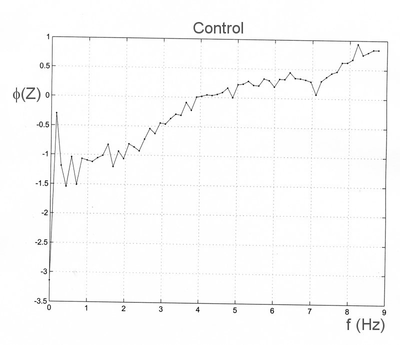
The very large peak at f = 8.3 Hz is the result of noise. If you examine the value of the magnitude of the transform of U at this frequency, you will see that it is almost equal to zero. When it is divided into the transform of P it gives an unnaturally large value. The phases are
To a fluid dynamicist, the main problem with impedance analysis is its implicit assumptions of periodicity and linearity. We have already seen that physiological data are seldom stationary and so the assumption of periodicity is generally unrealistic. The assumption of a linear relationship between pressure and velocity (or flow rate) is also a stronge assumption. The only examples of flows with a linear relationship between pressure and velocity are Poiseiulle flow (steady, flow in a long, straight tube) and Darcy flow (flow through low porosity material such as rock or soil, where the Reynolds number of flow in the pores is very small).
Allied to impedance analysis are the transfer function methods. In a linear system, the response of the system can be represented by a transfer function. Once the transfer function is known, the response of the system to any input can be determined as the convolution of the input and the transfer function. The convolution operation is an integral operator that can be difficult to calculate directly. However, it can be shown that the Fourier transform of a convolution is equal to the simple product of the the Fourier transforms of the transfer function and the input function. Thus the response of any linear system whose convolution function is known if very easy to calculate using the FFT.
Recently this idea has been applied to determine the pressure in the ascending aorta. Researchers determined the transfer function for the arterial system in a large number of submects by measuring the central arterial pressure waveform invasively and the pressure waveform in the radial artery using the non-invasive aplanation tonometry method. They then calculated the average transfer function as a function of sex and age and bundled everything together into a computer based machine that has been sold widely. The machine purports to give the central arterial waveform from the measured radial artery pressure waveform.
One worry about this process is the assumption that patients in the clinic have an 'average' transfer function. Almost by definition, people in clinics are not average - if they were, they wouldn't be in the clinic being examined. The most important worry, however, is the assumption that the arterial system is linear. This needs to be tested thoroughly.
We have recently measured the arterial pressure waveform as a function of distance away from the heart in the dog under different conditionsl. The measurements were made using a catheter based pressure transducer which was advanced to the ascending aorta from the femoral artery. The pressure was measured over several respiratory cycles, the catheter was withdrawn 2 cm and the pressure waveform was again measured. This was done in steps of 2 cm from the ascending aorta to the femoral artery. The data shown are the ensemble average waveforms at each measurement site
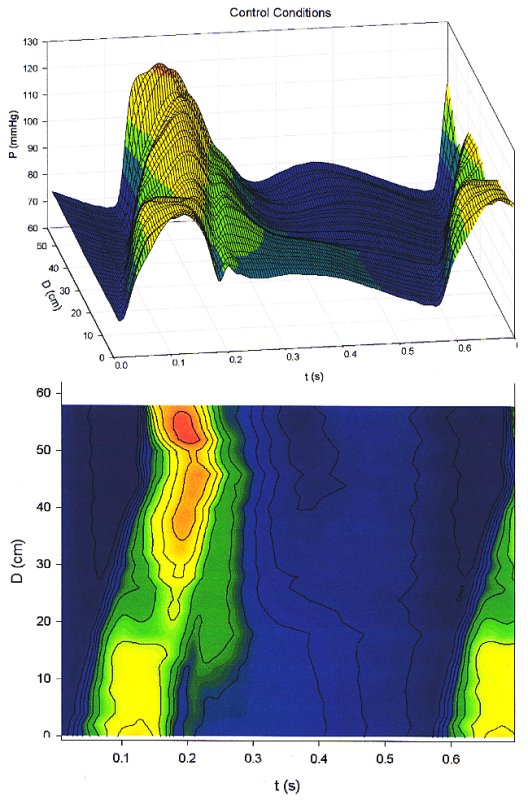
The top figure shows the pressure as a function of time and distance from the heart as a 3D plot. The bottom figure is the contour map of the same data. Notice the peak pressure decreases from the ascending aorta for a distance of about 20 cm and then begins to increase. The peak pressure is observed in the femoral artery where the peak pressure is significantly higher than it is at the origin of the aorta. Also notice that you can determine the wave speed in the aorta from the slope of the contours in the contour plot.
Similar measurements were made in a dog during infusion of methoxamine, a vasoactive drug with some inotropic affects.
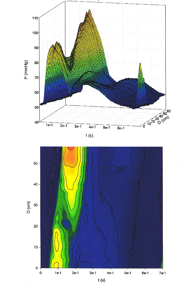
Note the enhancement of the decrease in peak pressure with distance and the ensuing increase with distance in the distal aorta. The enhancement of the peak pressure in the femorals is even larger than that observed in the control dog.