On a number of occasions we have used the concept of dimensional homogeneity to test the validity of a mathematical expression of a physical law. In this chapter we will explore this concept more thoroughly and show how useful it is; in addition we will show how the concept may be used in the derivation of physical laws.
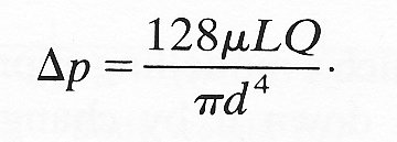
In most cases, it is easy to see how we may convert a law into dimensionless form; such a regrouping often tells us something of the relationship between the physical variables involved in the law. For example, let us again look at Poiseuille's law (Chapter 5, §5.1). As a dimensional statement we recognize it as
If we define U by
![]()
and substitute for Q and divide both sides by the product pU2, then we may write the equation in the dimensionless form
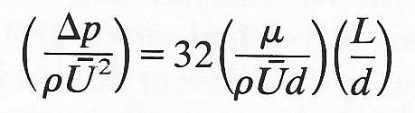
or substituting for Reynolds number (Re)
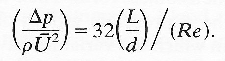
With Poiseuille's law written in this dimensionless form we are led to the concept of similarity. Thus we can look at the flow conditions in two pipes of differing diameters, with fluids of differing viscosity flowing at different flow-rates. It is possible that flow conditions will be 'similar'; and this will be so if respective conditions are such that each of the groups (Dp/rU2), (L/d) and Re are the same. If one or more of the groups are different in magnitude then the flows will be dissimilar.
The concept of similarity gives us great power in experimental research, for it enables us to design and interpret experiments on scale models of the system we would really like to study.
If the real system is inconveniently large or small, we may scale quantities appropriately so that it is possible to study a similar dynamic condition in a model of reasonable size. For pipe flow studies we can scale down very large tubes to a convenient size, and very corrosive materials which it would be unpleasant to handle in a laboratory may be replaced by safer materials such as air, water or oil of the appropriate viscosity and density.
Prototype aircraft designs do not have to be flown to test their aerodynamic proficiency; it is possible to test small-scale models in wind tunnels. By adjusting the wind speed in the tunnel and the model orientation, it is possible to predict how a full-scale aircraft would react to dynamically similar changes in flight conditions.
Again, the microcirculation is so small in physical size that quantities we would like to measure such as pressure drop are too small for instruments to deal with readily. For this reason large-scale models of the microcirculation have often been constructed. In fact much of our knowledge of the mechanics of the microcirculation has been derived from studies on enlarged models (see Chapter 13).
However, when we apply such a modelling approach to any problem we must be aware that it will break down if by changing the scale of one of the parameters beyond reasonable limits we need other additional laws to describe conditions. For example, it is easy to envisage experimental situations in fluid flow where the pressure gradient is increased to such a degree that the fluid must be treated as compressible, and the simplifications associated with incompressibility are no longer valid.
We may also use dimensional analysis and dimensionless groups when studying complicated problems, to tell us which groups of variables should be held constant at any time and to what extent other variables should be altered. It helps greatly in the presentation of results since they can be best presented as plots of data grouped in dimensionless form. Then we can see the response of the system to changes in the appropriate groups of variables without being concerned about the units in which the variables have been expressed. This is particularly valuable if comparisons are being made of results obtained by different workers.
The examples of scaling described above relate to mechanical processes; it is, however, quite possible to scale gross physiological behaviour of animals. For instance, we can scale such things as metabolic rate, anatomy and body chemistry as functions of, say, body size. Such correlations can be impressive in their closeness; often there are also deviations whose existence can be instructive.
A simple and perhaps surprising relationship is that between body weight and shape. It can be seen for vertebrates (for an enormous range of weight) that the outer surface area is about twice that of a sphere with the same volume (Fig. 6.1).
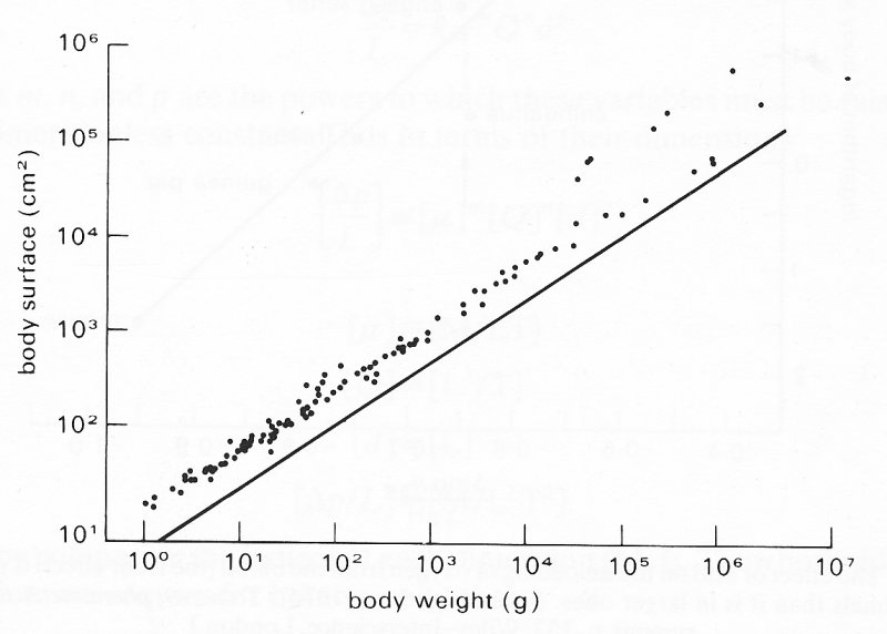
Fig. 6.1. Body surface area of vertebrates in relation to body weight. The solid line represents the surface area of a sphere of density 1 g em-3. (From Lightfoot (1974). Transport phenomena and living systems, p. 348. Wiley-Interscience, London.)
The volume of individual organs in relation to body volume also shows remarkable constancy in mammals. Thus the volume of the heart is approximately 0.5 to 0.6 per cent of body volume; however, the hearts of greyhounds and race horses are exceptionally large. Indeed, when one considers the cardiovascular requirements of these animals, this might be expected.
The effect of body size on mammalian blood takes two forms. First, the haemoglobin of smaller animals releases oxygen more readily at a given pH, thus helping to maintain the increasing metabolic rate as size decreases. Secondly, the effect of pH decrease (or increase in p(CO2)) on the oxygen release - the Bohr Effect - is greater for smaller animals, as can be seen from Fig. 6.2.

Fig. 6.2. The effect of acid on the unloading of oxygen from the blood (the Bohr effect) is greater in small animals than it is in larger ones. (From Lightfoot (1974). Transport phenomena and living systems, p. 352. Wiley-Interscience, London.)
There are two interesting deviations on this figure. It can be seen that the Bohr effect is unusually large in the horse - a creature accustomed to the exertion of running for long periods. The chihuahua is a relatively new breed of dog developed for fashion, not function, and it exhibits a small Bohr effect; this result of rapid selective breeding would appear to be a distinct disadvantage.
In many problems we can guess which variables are involved, but unless we know the laws governing the process, it is not immediately obvious how they are related. By applying the principles of dimensional analysis we can often find out. We know that for any physically realistic description of a process the equation must be dimensionally homogeneous, and thus we must group the variables in such a way that homogeneity is achieved. The technique for doing this is known as the indicia! method and two simple examples will serve to show how it may be used.
For the first example let us look again at the problem of flow in a tube. We know that the pressure gradient along the tube (Ap/L) will depend upon the diameter of the tube d, the volume flow-rate Q, and the fluid viscosity (JL. If we are concerned with flow far from the entrance of a straight tube we know that the fluid elements experience no acceleration. Thus we are not concerned with fluid inertia, and fluid density is not relevant.
Hence we can say that the pressure gradient is a function of viscosity, volume flow-rate and tube diameter or

Let us assume that the gradient is a single function of these variables, and let us further assume that the variables are related as follows:

where m, n, and p are the powers to which these variables must be raised and k is a dimensionless constant. Thus in terms of their dimensions

but
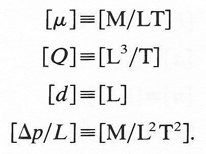
Thus by comparing the indices of each dimension (M, L, T) on both sides of the equation, we require for homogeneity that
for mass 1 = m
for length -2 = - m + 3n + p
for time -2 = - m - n.
Solving these three equations simultaneously, we have
m = 1, n = 1, p = - 4
or
![]()
Thus the only dimensionally homogeneous relationship between the variables is
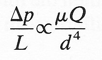
or

and this must be the form the relationship actually takes. This of course we recognize as Poiseuille's law, where, by theoretical calculation, the constant k has been shown to be 128/p.
As a second simple example we may consider the case of very slow flow past a sphere (see Chapter 5, §5.9). In this case again we may ignore the effects of inertia and consider the viscous effects only. The force F exerted by the fluid on the sphere will depend upon the size of the sphere (radius a), the velocity u of flow past the sphere and the fluid viscosity m.
Thus
F = f (a,u,m).
Considering the dimensions of the variables
[F] = [a]m[u]n[m]p
but
[F] = [ML/T2]
[a] = [L]
[u] = [L/T]
[m] = [M/LT].
Comparing indices for each of the dimensions M, L, and T
l = p
1 = m + n - p
-2 = - n - p.
Thus
m = l, n = 1, p = 1
and therefore
![]()
If we now consider the particular case of a sphere slowly falling under the influence of gravity through a viscous fluid (for example, the slow sedimentation of fine sand particles in water), then the force exerted by the sphere will be proportional to its volume and the difference in density between the sphere and fluid (B - F). Then
![]()
Thus
![]()
or
![]() (6.1)
(6.1)
This in fact is Stokes' law for slow flow round a sphere. The value of the constant k in this equation can be shown to be 2/9.