In order that we can understand the flow properties of biological fluids such as blood which may exhibit non-Newtonian properties it is first necessary to discuss the behaviour of simple or Newtonian fluids. Let us look at the flow properties of a simple liquid like water in a very long horizontal pipe. Imagine that this pipe is circular in cross-section and is d units in diameter (Fig. 5.1).
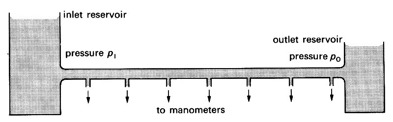
Fig. 5.1. Schematic drawing of a long, straight, horizontal tube with steady flow showing inlet and outlet reservoirs and the regular location of lateral pressure tappings.
Its entrance and exit are connected to large reservoirs so that the pressure drop between the ends of the tube may be maintained constant and a steady flow of water through the pipe achieved. Small side hole, or lateral, pressure tappings are made in the pipe at frequent intervals along its length and these tappings are connected to a series of manometers. It is thus possible to measure the pressure drop per unit length or pressure gradient along the pipe.
If the pressure at the inlet to the pipe is p1 and that at the outlet p0, then we shall observe that, as p1—p0 (or Dp)* [*The symbol Dp means the difference in pressure between any two stations 1 and 2; thus it is a form of shorthand for p1 - p2. In general DM means the difference between the value of the property M at stations 1 and 2.] is increased by raising the level in the upstream reservoir, so is the flow-rate Q through the pipe. However, if we look at the distribution of the pressure drop along the pipe we see that initially the pressure falls very rapidly with distance from the entrance, but after a long distance, which may be as much as 100 d, the pressure falls linearly with distance (Fig. 5.2 (a)).
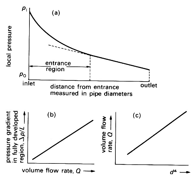
Fig. 5.2. (a) The variation in local lateral pressure with distance down the tube. Initially, in the entrance region, the pressure falls rapidly with distance but far from the entrance the pressure falls linearly with distance, (b) The linear variation of the pressure gradient (Ap/L) in the region remote from the entrance as a function o{ the volume flow-rate Q through the tube. (c) The linear increase in flow-rate Q with increasing pipe diameter to the fourth power d4 at a constant applied pressure gradient in the region remote from the entrance.
The region in which the pressure is falling relatively rapidly is called the entrance region of the pipe. The flow remote from the entrance is said to be fully developed or established. In the fully developed section of the pipe the pressure falls linearly with distance, i.e. the pressure gradient Dp/L (pressure difference between two stations distance L apart divided by L) is constant. In this region also the pressure gradient increases linearly with flow-rate 0 (Fig. 5.2 (b)).
If we perform the experiment using pipes of various diameters d, we see in the fully developed section for a given pressure gradient that the volume flow-rate Q increases very rapidly with diameter. In fact 0 increases with d4 (Fig. 5.2 (c)). The corollary of this is that if we wish to maintain a given volume flow-rate through pipes of successively decreasing diameter, then the applied pressure gradient must be increased by the fourth power.
There is a further instructive experiment that we may perform which will demonstrate how the velocity of flow varies across any cross-section in the fully developed region of the pipe, i.e. it demonstrates the velocity profile of the flow. Suppose that we rapidly inject a narrow streak or filament of dye across the pipe as in Fig. 5.3;
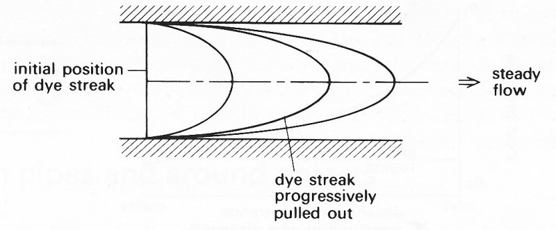
Fig. 5.3. The effect of flow progressively stretching a dye streak initially injected as a straight line across the tube. The successive lines indicate the position reached at different times after injection.
as the flow proceeds downstream, this filament will be transported with it and will become stretched out as shown. Each small elemental length of the streak will be transported downstream at the rate of the local fluid velocity. Thus if we record the position of the dye streak at various times after injection, it is possible to compute the velocity profile. It is possible also to introduce small blobs or fluid packets of marker dye at various radial distances from the axis and to watch their movement in a similar manner. Each isolated element will be seen to move with the local fluid velocity as before. It will also be noticed that as it is transported the packet will retain the same radial position; it will not drift towards the axis or wall nor will it corkscrew or spiral down the tube. This indicates that the flow is unidirectional or axial. It is also symmetrical, that is, the flow at any given radial distance from the axis is the same no matter which radial ray we look at. This is called axisymmetric flow. As will be confirmed below theoretically, the velocity profile is in practice parabolic in shape with the maximum velocity along the axis, the velocity reducing progressively to zero at the wall.
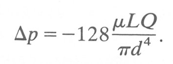
It was Poiseuille in 1840 who, as a first step towards understanding the mechanics of the circulation, published a quantitative study of the flow properties in a pipe very remote from the entrance, and flow conditions in this region are now named after him. In addition to varying the flow-rate and tube size, Poiseuille also studied the effect of viscosity on the flow conditions. He found that as viscosity was increased so was the pressure gradient necessary to maintain a given flow-rate. On the basis of his experiments Poiseuille carried out a theoretical analysis of the flow and derived his famous law for steady flow in a pipe remote from an entrance:
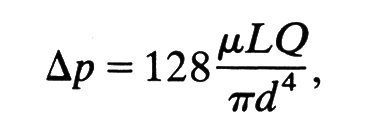
where m is the fluid viscosity.
By considering the physical processes operating on the fluid flowing in this region of the pipe it is possible to show how Poiseuille 's Law was derived. To do so we may apply a force balance to the fluid in a section of the pipe. In Chapter 4 we wrote down the groups of forces we need to consider in any force balance (Equation (4.5), §4.4). In Poiseuille flow we are considering a steady flow in a straight line so no fluid is subjected to any accelerations, and the left-hand side of Equation (4.5) is zero. In addition, if we consider flow in a horizontal pipe, gravitational forces are not relevant and the body force term is also zero. Thus we are left with a force balance which says:
viscous force = - pressure gradient force.
Consider the flow to be like a set of thin concentric shells of fluid sliding over one another as shown in Fig. 5.4,
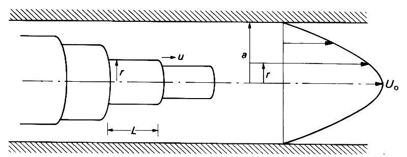
Fig. 5.4. Poiseuille flow in a straight tube showing the parabolic distribution of velocity.
and let us look at the force balance on a shell of inner radius r and thickness dr. If the pressure drop over a short length L of the cylinder is Dp, then the net pressure force acting on the shell is given by the product of the pressure difference and the cross-sectional area of the shell:
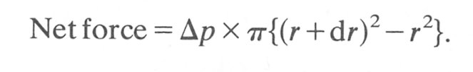
Since dr is small:
![]()
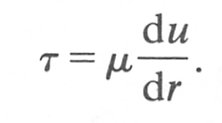
The net viscous force acting on the shell will be given by the difference in shear force on the two surfaces of the shell. The shear stress at any radial position is given by (§4.3)
The rate of change of stress with radius is given by
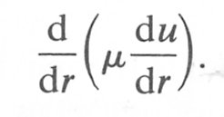
Thus for small changes dr in radius we can say that the difference in shear stress at the two radii r and (r + dr) is given by
and the net viscous force on the shell is:
Hence equating the two forces on the shell
Thus
If we now integrate this equation (i.e. sum the effects of all the shells) we obtain Poiseuille's law (Equation (5.1)). We can also show that
 (5.2a)
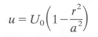
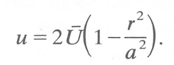
where u is the velocity at any radial position r, U0 is the centre line velocity, and a = 1/2d is the tube radius. We may define the average velocity U of the fluid as
![]()
and it can be shown that Equation (5.2a) can be rewritten as
 (5.2b)
Thus we can see that the velocity distribution in the pipe is parabolic, which explains the dye experiments above, and that the centre line velocity is twice the average velocity of the fluid.
Because the distribution of the velocity across the pipe is parabolic, it follows that the velocity gradient or shear-rate is a linear function of radius:
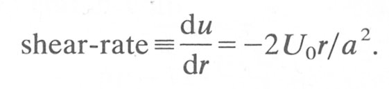
At the axis (r = 0) the velocity gradient is zero and it increases linearly to the wall where it has a maximum value of 2U0/a. Thus the viscous shear stress at the wall is given by t . 2U0/a and is the maximum shear stress.
It is possible also to derive Poiseuille's law on the basis of an overall force balance on a section of the pipe of diameter d and length L. If the difference in driving pressure between the two ends of the section is Dp, the net pressure force applied to the fluid is given by
![]()
The force opposing the applied pressure force is equal to the total viscous retarding force operating over the surface of the cylinder. Thus
Viscous force = viscous wall stress x tube surface area W
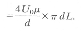
Since no other forces are acting
![]()
but Uo=2U and U=4Q/pd2, thus, substituting in the above equation and rearranging,
This can be seen to be Poiseuille's law as given in Equation (5.1). In the equation as expressed above there is a minus sign in front of the right-hand side of the equation. Strictly this is necessary because we are dealing with vector quantities, but the sign can be dropped for convenience as we clearly know the direction in which the forces are operating.
The application of this overall force balance to the flow is instructive for it demonstrates that it is the viscous retarding force operating at the tube wall which effectively opposes the flow.
It must be emphasized that Poiseuille flow conditions are pertinent only to regions of a straight pipe which are a very long distance from the entrance and remote from any sources of disturbance such as bends or constrictions. If we now look at the distribution of velocity of the elements of fluid flowing through any cross-section in the pipe nearer to the entrance, we can see that there are changes with distance along the pipe. At the entrance, all the elements of the fluid are moving with the same velocity and therefore have a uniform or flat velocity profile. However, the fluid which comes into contact with the wall of the pipe is forced to be motionless because of the 'no-slip' condition (see §4.3). Immediately, a gradient in velocity is established between the motionless fluid at the wall and the adjacent fluid elements just within the core. As the flow proceeds along the tube, viscosity progressively modifies this initial blunt profile as shown in Fig. 5.5.
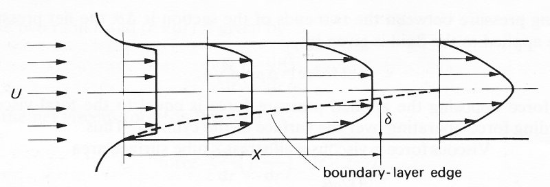
Fig. 5.5. The change in velocity profile with distance along the tube in steady flow indicating the growth of the boundary layer whose thickness is d distance X from the entrance. The initially flat profile becomes progressively modified to the established parabolic profile a long distance from the inlet.
The original high velocity gradient at the wall becomes reduced and progressively more of the core fluid becomes sheared. It is essential to realize that, at the same time, the central portion of the flow is accelerated to maintain the constant flow-rate through any cross-section. The gradient in velocity initially to be seen only near the wall becomes evident across progressively more of the tube radius. Ultimately, the velocity can be seen to vary across the whole cross-section of the pipe; it is maximum along the centre line and diminishes progressively towards the walls; the velocity profile is parabolic and Poiseuille flow is set up. Once this fully developed profile is achieved it does not change any further with distance downstream.
The progressive development of the velocity profile in the pipe is related to the changing pattern of pressure gradient with distance down the pipe.
In the entrance region, where the velocity profile is changing with distance, the pressure gradient is initially very high; however, further downstream, where considerable adjustment of the profile has already occurred, the gradient is less. Ultimately the pressure gradient becomes constant, at its lowest value, in the region of the pipe where flow is fully established. If the viscous retarding force at any cross-section before the flow becomes fully developed is calculated, it will be seen to be less than the applied pressure driving force. The excess driving force is taken up in accelerating the flow.
The fundamental difference between entrance and fully developed flow in a pipe is that in the entrance region fluid elements experience acceleration (positive near the tube axis and negative or retarding near the wall). However, since flow is steady, there is no change in velocity with time at any station in the pipe, i.e. there is no local acceleration. None the less individual elements of .fluid are accelerated or retarded as they move downstream along the pipe. This is an example of convective acceleration.
In general, flows contain both local and convective accelerations, and the forces (inertial forces) required to overcome the inertia of the fluid and provide these accelerations must be considered. These are the forces which comprise the left-hand side of Equation 4.5, §4.4.
As we have seen, in the entrance region, the velocity profile near the wall is continuously changing. The viscous drag exerted by the wall of the tube on the fluid nearest to it is progressively transmitted to regions of the fluid further away from the wall. This is the. result of the effects of the viscosity of the fluid.
Very near the entrance to the tube the thickness of the layer in which the fluid viscosity is acting is very thin (Fig. 5.5); outside this the velocity profile is almost flat and viscous effects are small. As the flow proceeds down the tube, the thickness of this layer in which viscosity is acting increases. We call this layer a boundary layer.* It characterizes the region in which viscosity plays an important role in determining the flow properties. [*Definition of boundary layer thickness: The boundary layer is that region of fluid in which the velocity is increasing with distance from the wall. Very near the wall the velocity changes very rapidly with distance, but far out in the layer it changes very slowly to the free stream velocity U0. For practical purposes we state that the boundary layer thickness is that distance from a solid surface at which the local velocity u reaches 0.99 U0.]
Boundary layers are established not only within tubes, but whenever a real fluid flows over any solid surface, for example, near the bed of a river or along the hull of a ship. If, instead of forcing a fluid to flow over a body, we pull that body through the fluid, we shall of course still establish a boundary layer over its surface. Thus if we look at the distribution of velocity around a body falling through water at a fixed speed, the boundary layer will look exactly the same as if we had made the water flow past the body at the same rate. It is only the relative motion of the body and fluid which is important. All real fluids demonstrate these characteristics but the details of the velocity profile within the boundary layer will depend upon the viscous properties of the fluid and we should not expect the profile to be the same for Newtonian and non-Newtonian materials.
We will now consider the rate at which the boundary layer grows with distance along the pipe; it depends upon the balance between the inertial forces and the viscous drag forces in the region of the wall.
Let us consider a small element of fluid in a region of varying velocity (Fig. 5.6).
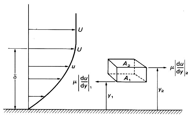
Fig. 5.6. A force balance on an element of fluid within the boundary layer.
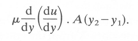
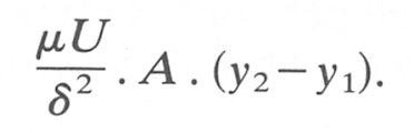
The tangential or shear stress on surface A1 (area A) is m|du/dy|1. Similarly the shear stress on A2, (also area A) is m|du/dy|2 . These two stresses will be slightly different in magnitude because of the change in velocity gradient in the region (see Fig. 4.7). The net viscous force on the element will thus be given by the change in stress with distance y from the wall:
The viscous forces on the element must balance the inertia forces. The inertia force term is given by
p x convective acceleration x volume of element,
where r is the fluid density and the volume of the element is A(y2-y1).
If we equate the two forces on the element and attempt to solve the problem mathematically, it will be found that there are not yet mathematical techniques available to solve the equation analytically. It is possible to obtain numerical solutions for particular problems only by using the digital computer. Commonly in fluid mechanics, in order to obtain an idea of the scale or magnitude of the process we are interested in, we give scales to the determining variables corresponding to their magnitude. (We shall see later, in Chapter 6, that this is an example of the techniques of dimensional analysis.)
Thus to obtain an estimate of the magnitude of the viscous force we may relate it to the local thickness of the boundary layer (5) and the free stream velocity U. Then the viscous force is proportional to
Again we may give the inertial force a magnitude scale. If the boundary layer thickness is considered at a distance X from the entrance to the tube, then the time scale for fluid to reach X from the entrance (the convection time) is of the order of X/ U. The convective acceleration of the fluid at the location X is then scaled as U/(X/U) or U2/X.
If we now equate these two scaled forces, we obtain
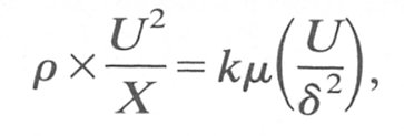
where k is a numerical constant whose size we must determine experimentally. Thus we can say
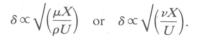
From Equation (5.3) we can see that the boundary layer grows with distance along the pipe as the square root of distance (see Fig. 5.5), i.e. as X1/2. Also as the flow-rate or free stream velocity is increased, the boundary layer becomes thinner at any location. The boundary layer thickness for a given flow-rate also increases with viscosity.
The analysis as described so far provides a very good estimate of the boundary layer thickness near the entrance to the tube, that is, when 8 is very small compared with the tube radius. However, when the boundary layer is fainy thick, its growth rate is modified because at any station along the tube the growth at one point on the tube perimeter is affected by the growth at neighbouring points round the perimeter at that cross-section. The effect of this interaction of adjacent parts of the boundary layer is somewhat to retard its development with distance. Nevertheless from Equation (5.3) we may obtain a scale for the length of tube required for the boundary layer to fill the tube and establish Poiseuille conditions. When the boundary layer fills the tube its thickness 8 equals the tube radius d/2. Then
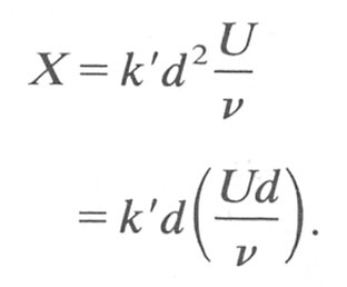
The term Ud/n is known as the Reynolds Number Re after the British scientist who first performed many important studies of flow in tubes, and it will be considered in greater detail below. The constant k' has been found experimentally to be approximately 0-03. Thus the entrance length X for steady flow in a straight pipe is given by
![]()
Hence we can see that for a tube of 2-0 cm diameter the entrance length would be approximately 60 cm for a Reynolds number of 1000 - this would be a typical situation for the aorta in man if it were a straight pipe and flow were steady at an average velocity of 0-2 m s-1.
Equation (5.4) is satisfactory for predicting the entrance length only when the Reynolds number is between 10 and 2500. When Re is very low (less than unity), inertia forces in the motion are negligible and the entrance length is about one diameter of the pipe. When Re exceeds 2500 the flow properties as they have been described so far break down—streamline motion no longer exists and turbulence may be observed (see §5.5).
Thus we shall see later that flow in the microcirculation can be considered as fully developed, but in large vessels it is of an entrance type - albeit complicated because of the geometry.
In the force balances we have used so far we have been concerned about the relative magnitude of the inertial and viscous forces operating on an element of fluid. In fact the ratio between these two forces is an important aspect of all flow problems.
In pipe flow U and d are the representative velocity and dimension of the flow. Therefore we can say that the magnitude or scale of the viscous force will be proportional to the product of viscosity and velocity gradient (= mU/d). Similarly the inertial force is proportional to the kinetic energy per unit volume (rU2) of the flow. The relative importance of the two quantities can then be expressed as the ratio
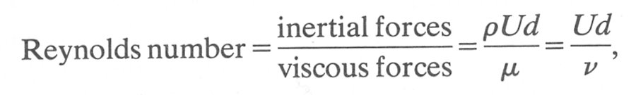 (5.5)
(5.5)
where n is the kinematic viscosity of the fluid (m/r). The Reynolds number Re is a dimensionless number and therefore its magnitude does not depend upon the units in which we express the various parameters provided we use a self-consistent set. Throughout this book we will regularly consider flows in terms of the Reynolds number. It is applicable for the characterization not only of conditions in a long straight pipe but of any flow situation. It is calculated on the basis of the characteristic velocity and dimension of the system.
Thus if we are considering flow round a sphere we may use the sphere diameter and approach velocity of the fluid. When the growth rate of the hydrodynamic boundary layer in a pipe was computed in the section above, we obtained Equation (5.3), which may be written as
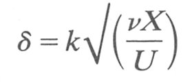
or
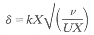
But the term UX/n can be thought of as the Reynolds number ReX for the flow based upon the characteristic length or distance X from the entrance of the pipe. We may thus rewrite Equation (5.3) as
![]()
When Re for a flow is much less than 1 we can say that the viscous forces dominate the flow and inertial forces can be ignored. For instance, in the microcirculation, which we will consider to be vessels less than approximately 100 mm in diameter, typical Reynolds numbers are less than unity and we can treat the flow as purely viscous. When Re is very much greater than 1 then inertial forces dominate the flow and viscosity has little modifying influence except very close to boundaries. Flow in large arteries and veins provides examples of this.
In 1883 Reynolds published important studies on the flow of fluids in long pipes. He obtained measurements of the pressure gradient along the pipe as the flow-rate was increased. At relatively low velocities, the pressure gradient was directly proportional to the flow-rate - this is as we would expect from Poiseuille's law (Equation (5.1)). However, at higher flow-rates, it became roughly proportional to the square of the flow-rate (Fig. 5.7).
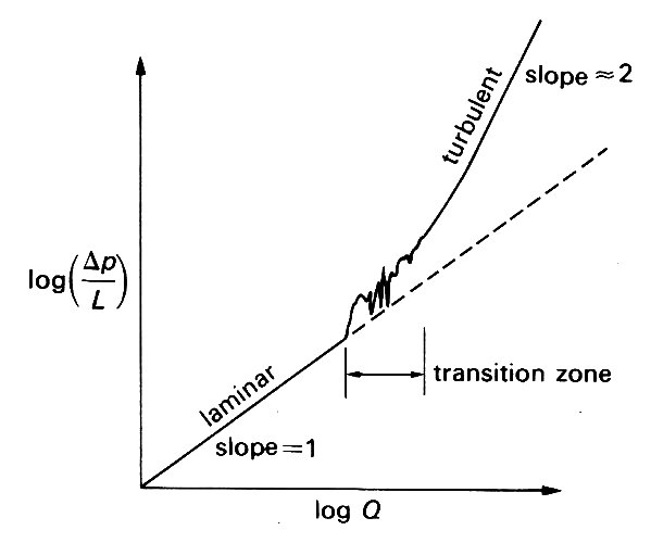
Fig. 5.7. The variation of volume flow-rate Q with pressure gradient Dp/L, plotted on a logarithmic scale, for steady flow in a long tube to indicate the changing relationship as the flow-rate is increased.
There was a range of intermediate flow rates where the relationship fluctuated with time: at one instant, the slope of the curve in Fig. 5.7 would be 1, then temporarily it would increase to nearly 2. If great experimental care was taken to ensure that flow entering the pipe was extremely steady and if the pipe was extremely smooth and straight, then the critical flow-rate at which the transition takes place from one state to the other could be made to occur at much higher flow-rates.
If we consider water flowing in a 1 cm diameter tube, the critical flow-rate at which the pressure-flow relationship changes is approximately 11 per min. This is a small flow-rate if we think about typical everyday flow situations like flow in the pipe to a tap or along a hose pipe.
Reynolds performed a second classic set of experiments in which he visualized what was happening within the flow. He studied the flow of water in a glass pipe and introduced a thin filament of coloured water into the main stream at the pipe axis far from the entrance, and observed its behaviour. At low flow-rates, the injected dye retained its identity and travelled along the pipe axis as a discrete filament. At higher flow-rates the dye streak was broken up and became mixed with the bulk of the water (Fig. 5.8);
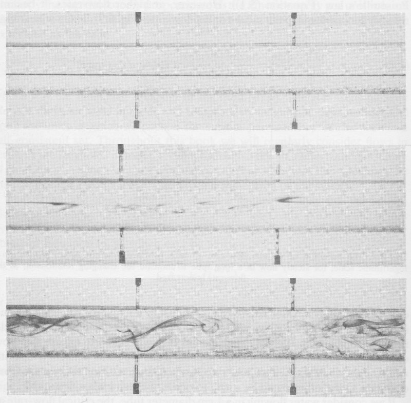
Fig. 5.8. The motion of a filament of dye in a long straight tube. Upper panel: the steady axial motion of a dye streak in a flow at low Re. Middle panel: At Re just greater than the critical value the steady laminar motion of the dye ceases and short bursts of turbulence can be observed. Bottom panel: At higher Re the flow becomes fully turbulent and random motion of the dye streak occurs.
the rate of mixing increased as the flow-rate was increased. At flow-rates just above the critical flow-rate, the dye streak could be seen to break up intermittently.
This random motion of the dye indicated that the flow was also flowing with violent random movements. Indeed, if a high speed cinefilm were taken of the motion of the dye and this were viewed at low speed, it would be seen that individual elements of dye would move randomly in time and all three dimensions of space. However, if we were to compute the time average velocity of packets of dye moving through any one point in a cross-section at some position in the pipe and then repeat the computation at other points in the same cross-section, we would see that there was a well denned time average velocity profile. The instantaneous random velocities of the elements would all be comparable with the local time average velocity. The increase in pressure gradient observed in the first set of experiments coincides with the onset of turbulent motion. The turbulent movements are associated with greater energy dissipation and therefore a greater rate of loss of pressure.
If the Reynolds numbers for the flows are computed, it will be seen that when Re is less than 2300 the flow is everywhere laminar, but when Re is greater than 2500 the flow shows continuous turbulence, which becomes more intense as the Reynolds number is raised. In the region between 2300 and 2500, transition occurs and intermittent turbulence is observed.
The dye streak visualization technique may be used to see how the turbulence in the flow develops with distance along the pipe from the entrance. Consider the set up shown in Fig. 5.1, where the flow-rate is increased to be sufficiently high for turbulence to occur. Dye streams may be introduced into the flow at various radial and axial positions and the fate of these streams observed as they are transported downstream. Just at the entrance the velocity profile will be flat with all elements of fluid moving at the same velocity. A short distance downstream viscous action will cause modification of the profile as described above, but the dye streams will still be intact and turbulence will not be present. Further downstream the dye streams will suddenly break up, showing that the flow is no longer laminar but has become turbulent. The first dye streams to break up will be those at the edge of the boundary layer, a very short distance afterwards the streams within the boundary layer and core also break up, showing the presence of turbulence. The established mean velocity profile far downstream will be different in shape from the laminar parabolic profile. The core has a much blunter profile and the velocity gradient at the wall is steeper; the peak velocity, on the axis, is approximately 1-2 times the average velocity.
The entrance length for a turbulent flow is less than that for laminar flow; its size may be estimated on the basis of the following equation:
![]() (5.7)
(5.7)
Again consider a long straight pipe with laminar flow in it. If now a slowly oscillating pressure gradient is applied to the flow it will slow down, stop and reverse direction, accelerate in that direction, then slow down again. If this takes place gradually enough then the flow will always have a parabolic velocity profile whose magnitude is proportional to the instantaneous flow-rate (Fig. 5.9).
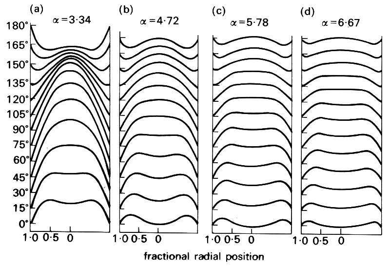
Fig. 5.9. Velocity profiles, at intervals of 15°, of the flow resulting from a sinusoidal pressure gradient in a long straight tube. The value of a in the left-hand panel (a) is sufficiently high to indicate that reversal of flow occurs near the wall whilst the core motion is still forwards. The motions in the remaining panels (b, c, d) indicate the progressive distortion of the profile at a values corresponding to the second, third and fourth harmonics of the basic frequency of oscillation in panel (a). (From McDonald (1974). Blood flow in arteries, p. 104. Edward Arnold, London.)
However, if the pressure gradient is cycled progressively more frequently, then the velocity profile becomes increasingly distorted (Fig. 5.9). The inertia of the fluid in the central core prevents the core from following the applied gradient of pressure and the amount by which it lags increases as the frequency of oscillation of the pressure gradient is raised still further. At the same time the amplitude of movement of the core fluid decreases. At very high frequencies we find that there is very little motion of the core, and all flow is constrained to a very thin region near the wall where viscous forces dominate and the flow is less sensitive to inertial forces.
The simplest form of oscillating pressure gradient that we can consider mathematically is the simple sinusoidal pressure gradient. In this case, the instantaneous pressure gradient (Dp1) is related to the maximum or peak pressure gradient (Dp0) by the relationship
![]() (5.8)
(5.8)
where t is time and w is the angular frequency (w = 2pf, where f is the frequency) of the oscillation. The instantaneous pressure gradient will vary with time in such a way that at time t = 0 it is zero; as time increases so will Dp1 increase to a maximum value of Dp0 and it will then decrease to zero again; as t increases further Dp1, will become negative and decrease to a value of -Dp0 and it will then rise again through zero and repeat the cycle. The period of time T over which one complete cycle of the pressure oscillation occurs is 2p/w. An extended discussion of sinusoidal functions is given in Chapter 8.
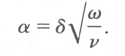
A very useful dimensionless parameter is the Womersley number a, which indicates the extent to which the velocity profile in laminar flow in a long pipe differs from the Poiseuille profile when the fluid is subjected to a sinusoidally varying pressure gradient of angular frequency w:
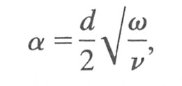 (5.9)
(5.9)
where d is the tube diameter and n is the kinematic viscosity (n = m/r). The parameter a may be considered as a kind of unsteady Reynolds number for the flow as it indicates the relative importance of inertial and viscous forces in determining the motion within the time scale of one period of an oscillation.
At low values of a (less than unity), the flow is 'quasi-steady' and the velocity profile is parabolic at all times, the magnitude of the flow-rate being determined by the instantaneous pressure gradient. Viscous forces dominate the flow and inertial forces can be neglected. At somewhat higher values of a the instantaneous velocity profile looks distorted (Fig. 5.9) because inertial forces have begun to influence the flow. Furthermore, the instantaneous flow-rate will no longer be the same as predicted on the basis of the instantaneous pressure gradient. The flow will lag behind the applied pressure gradient. We may describe this mathematically as follows. At low values of a, the applied pressure, as given by Equation (5.8), generates a flow-rate Q, which is determined by the instantaneous pressure gradient Dp1, and Poiseuille's law. Then
![]() (5.10)
(5.10)
where QST is the flow-rate obtained for the pressure gradient Dp0. At higher values of a (in the range approximately 1-3) the instantaneous flow-rate lags behind the instantaneous pressure gradient by an amount of time f and then Equation 5.10 becomes
![]()
i.e. the instantaneous flow-rate is given by the applied pressure gradient at the earlier time t - f. At even higher values of a (greater than approximately 4) inertial forces begin to dominate the flow to such an extent that not only does the phase lag continue to increase, but also the peak flow-rate QP becomes progressively less than predicted from the peak pressure gradient Dp0. The variation of both phase lag f and peak flow-rate with increasing a can be seen from Fig. 5.10.
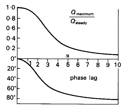
Fig. 5.10. The effect of progressively increasing a on the amplitude (upper panel) and phase (lower panel) of oscillatory flow resulting from a sinusoidally applied pressure gradient. The amplitude is expressed as the ratio of the instantaneous maximum flow-rate (QmaximumJ to the steady flow-rate (Qsteady) at the maximum driving pressure. (From McDonald (1974). Blood flow in arteries, p. 125. Edward Arnold, London.)
In the circulation, the value of a (based on the cardiac frequency) varies over a considerable range; thus in the aorta a can be larger than 10 whilst in a capillary it is of the order of 10-3. Furthermore, in the circulation and indeed in many practical flow situations, we are concerned not with Poiseuille flow but with rather more complicated velocity profiles. These may be either of an entrance type or profiles which are disturbed because of geometrical effects. In these cases it is inappropriate to calculate a on the basis of the diameter of the tube or vessel. The parameter should be calculated using, in place of the diameter, the thickness (d) of the hydrodynamic boundary layer which would have been present in steady flow, because in reality a is an estimate of the effect of oscillation in distorting the steady flow. Thus
Since the boundary layer thickness is always less than the tube radius (d/2) we can see that a will always be lower than anticipated on the basis of established flow conditions. However, in the circulation, it is not possible to determine d accurately and so values of a are always quoted on the basis of the vessel diameter.
So far we have only considered flows within tubes of constant cross-sectional area. In this section we shall look at the effects of flow through constrictions and then in the next section at the properties of flow around bluff bodies and in curved tubes.
Consider a long straight horizontal tube with a sudden rapid change in cross-sectional area (Fig. 5.11)
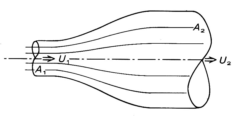
Fig. 5.11. Flow in a circular tube of expanding cross section from area A1 to area A2. Note that the velocity falls from U1 to U2..
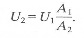
from area A1 to area A2. The fluid contained within the pipe is incompressible and is flowing with steady laminar motion, and for the moment we suppose that viscosity can be neglected. Clearly, as the fluid passes into the larger area tube, its velocity must fall since the volume flow-rate is the same in both sections:
![]() (5.11)
(5.11)
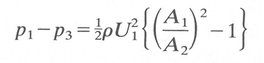
Since there is no viscosity, there is no dissipation of energy, and we may apply Bernoulli's theorem to the flow and make an energy balance between the two sections:
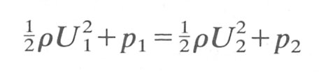
or
![]() (5.12)
(5.12)
But we know that U2 is less than U1, so the static pressure in the larger downstream area is greater than that upstream. The excess kinetic energy associated with the flow has been converted into static pressure. If the flow had been in the reverse direction we would have seen a decrease in static pressure on entry to the region of smaller cross-sectional area. If the fluid was real and of low viscosity then we could apply the same argument, because the pressure loss due to viscous action in a short section of pipe in that region would be very small compared with the pressures involved in the Bernoulli balance (Equation (5.12)).
On the basis of this last assumption, the Venturi Meter was developed for the measurement of flow. The meter as shown schematically in Fig. 5.12
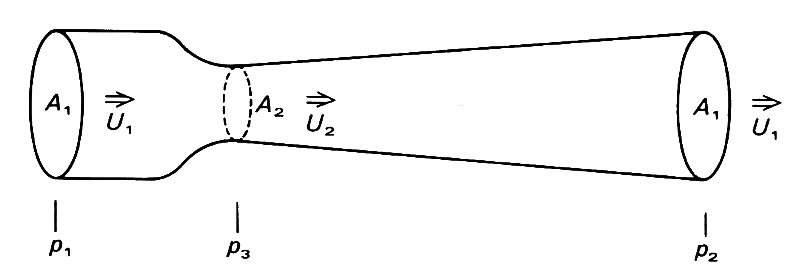
Fig. 5.12. Flow in a Venturi section where initially the tube cross-sectional area is decreased from 'A1 to A2, and then slowly re-expands to area A1. The pressure measurements p1, p3, and p2 are made upstream of the constriction, at its maximum and far downstream respectively.
consists of an initial contraction from the main tube cross-sectional area A1 down to a constricted throat of area A2, followed by a very slow expansion back to the original cross-sectional area. This expansion section is designed to have a divergent half angle of less than five degrees in order to avoid certain energy losses associated with flow separation, which will be discussed later.
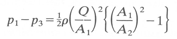
If we assume that there are no frictional losses, then from the above discussion we know that p1 will be greater than p3, but that pressure will rise again downstream till at the end of the divergent section the pressure will have recovered to p2, which should equal p1. However, in reality friction losses cause p2 to be slightly lower than p1, though if the meter is well designed, they will be small and may be ignored. The volume flow-rate Q may be calculated as follows. It is very important to note here that in this example we are not talking about the mass flow-rate but the volume flow-rate. If we confused the two we would derive inhomogeneous equations with inconsistency in the units. Using Equation (5.12) for an energy balance across the convergent section we have
![]() (5.13)
(5.13)
Also from Equation (5.11) we know that
![]()
i.e.
Substituting in Equation (5.13):
but Q = U1A1; then
or
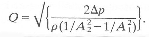
Thus we can see that provided the geometry is known, we may compute the flow-rate from the pressure drop across the convergent part.
The familiar laboratory water suction pump which fits on to a tap is a device designed rather like a Venturi meter. Water is forced to flow through a constriction, and the fluid acceleration causes a reduction in local static pressure; it is this which acts as the suction pressure for the pump.
If, after the constriction, the tube expands too rapidly, then the phenomenon of 'flow separation' occurs. When this happens there is no longer simple streamline motion across the whole of the cross-section. We find that there is forward streamline motion in the core of the tube, but that flow near the walls is sluggish and recirculation of fluid occurs as shown in Fig. 5.13. This separation is a consequence of the increase of pressure along this section (see above, §5.7). In a straight tube, pressure is falling in the direction of the flow and conditions are stable; again, in the convergent section of the meter, pressure is also falling, at an even faster rate. In contrast, in the expansion section of the meter the pressure is rising in the direction of motion and this is adverse to the flow. The effect of this adverse pressure force is to tend to retard the flow. In the core the inertia of the fluid opposes the retardation. However, near the wall the fluid velocity is small, because of the no-slip condition, and its inertia is very low, negligible in comparison with the viscous forces. As a result, when the adverse pressure gradient slows the fluid down, the flow near the wall ultimately reverses. When this happens, there is a drastic change in the nature of the boundary layer, which no longer remains thin and is said to separate. The large effect of separation of the flow in the core of the tube can be seen in Fig. 5.13.
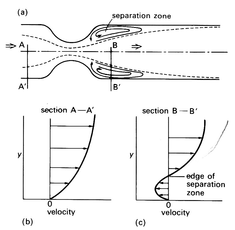
Fig. 5.13. Flow through a constriction followed by a rapid expansion downstream showing the region of flow separation (a). The sections at A-A' (b) and B-B' (c) show the velocity profiles at those stations. At the upstream station the flow is everywhere in the forward direction; at the downstream station fluid near the wall has motion in the reverse direction.
As long as the flow field is laminar, the degree of separation or the size of the zone and intensity of recycling flow will increase as flow rate is increased. The tendency for turbulent flows to separate is less strong than for laminar flows; thus turbulent flows can withstand more acute geometric changes than can laminar flows.
It is possible to produce constrictions in a tube which are much more severe than the above Venturi type; thus an orifice inserted into a tube causes severe flow changes. Let us look at the effect of introducing a sharp-edged orifice into a tube as in Fig. 5.14,
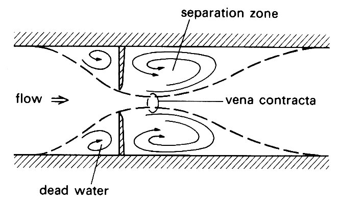
Fig. 5.14. Flow through an orifice showing that the flow continues to be constricted beyond the site of the obstruction, being of minimum cross-sectional area at the 'vena contracta'. Note also that separation occurs downstream of the orifice.
considering first steady laminar flow of a real fluid. As the flow approaches the constriction, the streamlines become bent and the flow accelerates. The fluid velocity in regions near the pipe wall and orifice is extremely low and these regions are effectively 'dead water' zones. As the flow passes through the orifice the jet continues to contract for a short distance further downstream till it reaches the 'vena contracta' where the effective cross-sectional area for flow is a minimum. Thereafter the flow diverges and ultimately fills the tube cross-section again. Immediately downstream of the orifice a separation zone can always be observed. It is characterized by a recirculating vortex-like motion. This results from the extremely rapid increase in cross-section immediately downstream of the orifice which produces a very large adverse pressure gradient for the flow. The flow emerging from the orifice does so effectively as a jet and the rate at which the boundary of the jet expands is relatively slow; as a result the separation zone extends some distance downstream.
If we measure the static pressure upstream of the orifice where flow is relatively undisturbed and compare this with the static pressure at the level of the vena contracta, the difference is slightly greater than that expected on the basis of an energy balance assuming no viscous effects. Downstream, the agreement is not nearly as good as in the case of the Venturi meter because of the viscous losses associated with the separation of the flow. If comparison of the static pressure far upstream is made with the static pressure some distance downstream, a large loss of pressure (or energy) will be observed. This results from the viscous dissipation of energy (in the form of heat) in the disturbed flow downstream of the orifice. At low flow-rates this occurs mainly in the separation zone, but at higher flow-rates the emerging jet becomes disturbed and turbulent in character. This adds considerably to the energy losses.
If we study the stability of flow through an orifice, it can be seen that at low flow-rates the emerging jet is laminar, but that at higher flow-rates it becomes disturbed and turbulent. If we compute the Reynolds number for the flow through the orifice, using the orifice diameter and the mean velocity of fluid flowing through it (from Equation (5.5)), it can be demonstrated that the change in character of the emerging jet occurs for an orifice Reynolds number of 300-400. Thus it is a very common situation to have an orifice in a pipe where there is nominally laminar flow in the main tube but a turbulent emerging jet.
In the blood circulation, coarctations and stenoses provide examples of constrictions to flow. The coarctation is perhaps most similar to the Venturi constriction and the stenosis to the orifice. The stenosis, the more common condition, is associated with a well-defined audible thrill which results from the noise created by the turbulence in the jet downstream of the orifice (see Chapter 11 and Chapter 12).
We have so far considered the properties of flow in a straight pipe; in a curved pipe further interesting phenomena can be observed. When fluid flows steadily and without turbulence round a bend, as in Fig. 5.15,
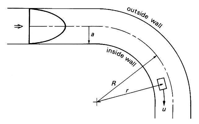
Fig. 5.15. Sketch of the centre plane of a curved tube, radius a, with Poiseuille flow entering. Radius of curvature of centre line is R. A fluid element of speed u, travelling along a path with radius of curvature r, experiences an inward acceleration u2/r.
every element of it must change its direction of motion. That is, it must have a component of acceleration at right angles to its flow direction. It follows that, like a single particle moving in a circle, every element must experience a force in that direction. In this case, the force must be supplied by a sideways pressure gradient, in the plane of the paper of Fig. 5.15, acting from the outside of the bend towards the inside. This will act more or less uniformly over the whole cross-section of the tube, and all fluid elements of a given mass will experience approximately the same sideways force to make them turn the corner. Therefore they will all be given the same sideways acceleration. But this means that faster moving elements will change their direction less rapidly than slower moving ones, because they have more inertia.* Thus the faster moving fluid which originally occupied the centre of the tube will tend to be swept out towards the outside of the bend, being replaced by slower moving fluid from near the walls. In consequence a transverse circulation or secondary motion is set up, as shown in Fig. 5.16. [*Alternatively, the magnitude of the lateral acceleration on any particle is u2/r, where u is the speed of the particle and r is the radius of curvature of its path; thus if the sideways acceleration is uniform, the paths of the slower moving particles must have smaller radii of curvature.]
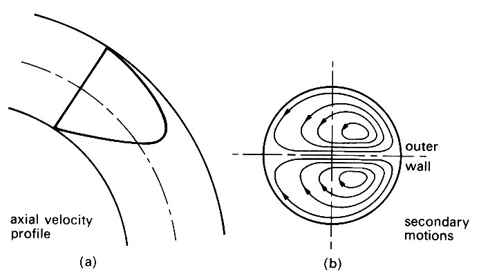
Fig. 5.16. (a) Distortion of the axial velocity profile as a result of tube curvature, (b) Projection of streamlines on to a transverse plane, clearly showing the form of the secondary motion.
At the same time, because the faster moving fluid has been swept to the outside of the bend, the axial velocity profile is distorted from its original symmetric shape, and the greatest velocities occur near the outside wall. This pattern of flow can be seen in a long, continuous bend, far from the entrance, where the flow is fully developed.
An important consequence of the distortion of the Poiseuille velocity profile, together with the presence of secondary motions, is that there are regions in the pipe, in particular near the outside of the bend (Fig. 5.16), where the shear-rate is considerably higher than in Poiseuille flow. High shear-rates mean that the rate of deformation of fluid elements is high, and hence that the rate at which mechanical energy is dissipated by viscosity is also high. Thus more work has to be done to force a fluid through a curved pipe than through a straight one. In other words, the pressure gradient necessary to maintain a given volume flow-rate is greater in a curved pipe than in a straight one. If a straight pipe has a single bend in it, and then continues straight, the flow downstream of the bend will contain secondary motions of the sort just described. These will gradually die away so that far downstream Poiseuille flow is once more established; the distance over which the secondary motions and distortions will persist is comparable to the distance for Poiseuille flow to be established at the entrance to a straight pipe. This entrance length is given by Equation (5.4).
When fluid enters a curved tube, a thin boundary layer is present on the wall as in a straight tube. In this case, however, the velocity profile in the core, where viscosity is unimportant, is not approximately flat, even if it is flat at the entrance itself. It is observed in experiments that the velocity of the fluid near the inside wall is greater than that near the outside wall (Fig. 5.17).
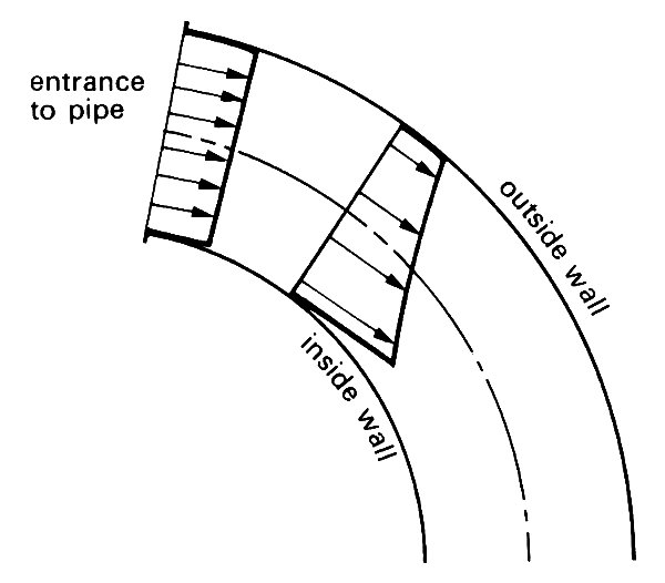
Fig. 5.17. Distortion of a flat velocity profile at the entrance to a curved pipe.
This can be explained by using Bernoulli's theorem (Equation 4.6, §4.7, which, when gravity is unimportant (e.g. when the flow is horizontal), states that the quantity
![]() (5.14)
(5.14)
is a constant along each streamline; as usual, p, r, u are the fluid density, pressure, and velocity respectively. Furthermore, because each streamline originates from a region where p and u are uniform, the constant has the same value on every streamline. Now, although no secondary motions are set up in the core in this region, because all fluid elements have approximately the same velocity, there must still be a sideways pressure gradient for the fluid to be forced round the bend. Hence p is greater at the outside of the bend than at the inside, and so for H to remain uniform, the fluid velocity u must be smaller at the outside than at the inside.
Secondary motions will not become important until a long way downstream, when the boundary layer is thick and the flow approaches its fully developed form. However, some recent experiments, combined with theoretical work, have shown that the details of the flow in the boundary layer, where weak secondary motions begin immediately, are affected by curvature. This has some interesting consequences, which can best be expressed in terms of the shear-rate. If the boundary layer were the same all round the tube cross-section, the skewed velocity profile in the core would result in the wall shear-rate being greater at the inside wall than at the outside. However, the incipient secondary motions in the boundary layer cause this distribution to be reversed after a distance along the tube of only about one diameter. From then on the maximum shear-rate occurs at the outside wall, as when the flow is fully developed.
Our main preoccupation so far has been to investigate the way fluids flow in tubes or systems of tubes, and it has become apparent that the most complex flow patterns arise through the interaction between viscous and inertial forces, in the entrance region of a tube for example. Another very good .example of this interaction is provided by the flow of a fluid past a solid body. We examine that example in detail here, both because it permits a deeper understanding of the general properties of a fluid in motion, and because many of the phenomena which arise are familiar from everyday experience.
We suppose that the body is totally immersed in the flowing fluid, so that there is no possibility of surface waves being generated; their presence would obscure the important features of the flow. For convenience, we also imagine the body to be a very long cylinder, with the fluid flowing past it at right angles, so that in the middle the influence of the ends is negligible, and there is no component of velocity parallel to the axis of the cylinder. This means that the flow in the middle is the same as if the cylinder were infinitely long; the velocity vector of a fluid element always lies in a plane perpendicular to the cylinder axis, and will depend on the position of the element in that plane, and on the time, but will be independent of the distance along the axis of the cylinder. We say that the flow in this case is two-dimensional; it is much easier to visualize than a fully three-dimensional flow. Let us further suppose that all other boundaries of the region containing the fluid are so far away that they have no influence on the flow, so that this region is effectively infinite. Finally, we shall at first consider only a cylinder of circular cross-section, since that is a convenient shape, which has been the subject of many theoretical and experimental studies. As far as the flow relative to the body is concerned, it is irrelevant whether the fluid is moving past the body (like the wind blowing past a building) or whether the body is moving through the fluid (as an aeroplane moves through the air, or a grain of sand sinks to the bottom of a pool). The flow is normally easier to visualize with the body at rest, although sometimes the other point of view is more helpful. We shall be examining situations where the body has a constant speed relative to the fluid far away from it. This means that the flow as a whole is steady when the body is taken to be at rest, but is unsteady when the body is moving in a fluid at rest far away.
First of all, we consider a hypothetical fluid with no viscosity, and temporarily abandon the no-slip condition. This means that the boundary layers which we would expect to occur on solid boundaries (see §5.3) are absent in this case. Their influence will be considered below. Suppose that the cylinder is at rest, and that far away from it the fluid flows forward uniformly with, say, speed U (Fig. 5.18).
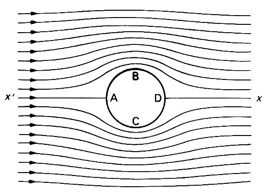
Fig. 5.18. A plane perpendicular to the cylinder axis, showing the streamlines (particle paths) for steady flow of an inviscid fluid past the cylinder. The velocity far from the cylinder is uniform, and everywhere parallel to the line x'x. A and D are stagnation points; B and C are points where, in the absence of viscosity, the fluid speed is greatest.
Nearer the body, however, the passage of some fluid is blocked; this fluid is retarded, and forced to flow round the sides of the body.
The paths of fluid elements initially far upstream of the body would approach the cylinder, be deflected above and below as shown in Fig. 5.18, and return to their original paths far downstream. In steady flow, fluid elements move along the streamlines of the motion (lines everywhere parallel to the velocity vector; see §4.7) and therefore Fig. 5.18 is also a diagram of the streamline pattern. (Alternatively, if the cylinder is thought of as moving, it has to push fluid out in front of it and draw it in behind it as it proceeds, and a flow pattern is set up like that depicted in Fig. 5.19.)
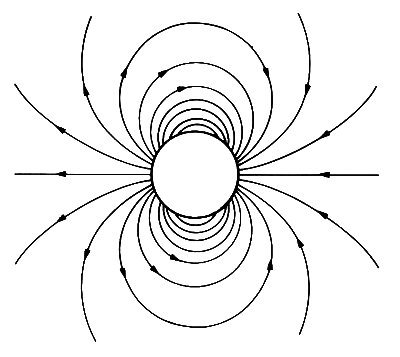
Fig. 5.19. A diagram of the (unsteady) streamlines set up by the motion of the cylinder in a fluid otherwise at rest. Fluid is pushed to the sides in front of the cylinder, and moves in behind it again when it has passed.
It is easier - because less energy is required - for the fluid to flow round the sides of the cylinder like this than, for example, for an infinitely long column of fluid to be pushed in front of and pulled behind the cylinder.
There is one streamline which divides the fluid flowing above the cylinder from that flowing below. At the point where this line meets the cylinder the total velocity must be zero although the no slip condition is not applied: the normal component of velocity is zero because fluid cannot cross a solid boundary, and the tangential component is also zero because, if it were not, the fluid there would be flowing one way or the other round the cylinder. This point, A in Fig. 5.18, is called a stagnation point. From Bernoulli's theorem (Equation (4.6), §4.7) we know that the pressure at A exceeds the pressure far away, where the flow is uniform (let this pressure be po), by an amount equal to 1/2rU2; this excess pressure can be thought of as providing the force required for the deflection of the other fluid. The velocity of a fluid element which passes close to A, and therefore has near-zero velocity there, must necessarily increase as it is forced sideways by this excess pressure towards the widest part of the cylinder, and experiences an acceleration. The streamlines are closer together in this region than they were far upstream, indicating that the velocity there is greater than U. In fact the velocity of fluid at B or C (Fig. 5.18) is equal to 2U; all fluid particles are accelerated over the forward half of the cylinder, until they pass the widest part. By Bernoulli's theorem, the pressure at B or C is less than po by an amount 3/2rU2. When there is no viscosity, the flow over the rear half of the cylinder is symmetrical with that over the forward half. The fluid particles are retarded, the pressure along the surface of the cylinder rises (to exceed p0 by 1/2rU2 at D again), and far downstream the uniform flow is once more achieved.
The symmetry of the flow leads to the prediction that the net force on the cylinder is zero. In fact it can be proved mathematically that no body in a uniform stream of inviscid fluid experiences any force in the direction of the stream. This prediction, which was first made by the French philosopher d'Alembert in 1752, is irreconcilable with the everyday observation that all bodies moving through fluids experience some resistance or drag, even when the numerical value of the coefficient of viscosity is very small (m = 0.00181 N s m-2 in air at 20°C, 0.1 N s m-2 in water at 20°C). This difficulty, known as d'Alembert's paradox, was a source of great concern in the nineteenth century. Its resolution lies in the fact that all fluids are viscous, and it turns out that however small m is, the presence of viscosity distorts the flow pattern so much that the drag is considerable.
Consider now a real fluid, whose velocity far from the stationary cylinder (of diameter d) is U. The Reynolds number is then equal to Ud/n (where n, equal to m/r, is the kinematic viscosity of the fluid). When this is very large, we expect inertia forces to predominate over viscous forces everywhere in the flow except near the boundaries, where the no-slip condition must be applied. We might therefore hope that the flow would be very similar to the flow of an inviscid fluid, except near those boundaries. Fluid elements will be retarded as they approach the stagnation point A (see Fig. 5.18), and accelerated again over the forward half of the cylinder. This time, there is a thin region near the walls across which the fluid velocity falls to zero, as required by the no-slip condition, and we can recognize this region as a boundary layer (see §5.6). It will be thinnest at the front of the cylinder (near the point A), but will remain quite thin all the way round to B and C, since the velocity outside it increases with distance along the cylinder surface. (As we have seen, by Equation (5.3), the thickness of a boundary layer increases as the square root of the distance along the boundary, but decreases as the square root of the velocity of fluid outside the layer.) Once the fluid has passed the widest part of the cylinder, however, it begins to be decelerated, and the pressure begins to rise, as described above for an inviscid fluid. This rise in pressure imposes an adverse pressure gradient on the boundary layer flow, and, as in a rapidly diverging tube, this causes the flow near the wall to come to rest and reverse (Fig. 5.20). From the point where reversal first occurs, the region in which the flow does not resemble that in an inviscid fluid, because viscous forces are important, is no longer confined to a thin boundary layer. Separation of the boundary layer has occurred (§5.7). This prevents complete recovery of the pressure from being achieved, so that the pressure behind the cylinder is much lower than that in front. Thus the body must experience a considerable drag, however large the Reynolds number. The measured distribution of pressure round the surface of the cylinder at Reynolds number 1.1 x 10⁵ is shown in Fig. 5.21, and is compared with the corresponding distribution for an inviscid fluid. It is the marked difference between the pressure distributions over the rear half of the cylinder which is responsible for a large part of the drag. The other contribution to the drag arises from the direct action on the wall of the tangential viscous stresses associated with the high rates of shear present in the velocity profile across the thin boundary layer (Fig. 5.20).
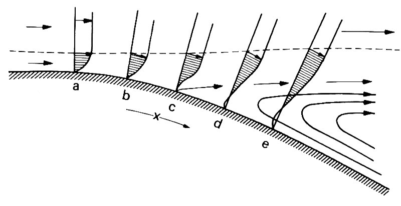
Fig. 5.20. Diagram showing the velocity profiles across the boundary layer, at different positions along the body surface. Note the region of reversed flow downstream of the point c of boundary layer separation.
For flow round a bluff body like a circular cylinder, however, this direct viscous component of drag contributes about 1 per cent of the total drag for Reynolds numbers above 100.
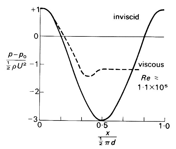
Fig. 5.21. Graphs of the pressure exerted on the cylinder, plotted against distance x from the front stagnation point, measured along the cylinder surface. The broken curve was measured when Re = 1.1 x 10⁵, while the solid curve is the theoretical curve for an inviscid fluid. It is the difference between these pressures at the back of the cylinder that is responsible for most of the drag. (From Batchelor (1967). An introduction to fluid dynamics, p. 340. Cambridge University Press.)
The character of the flow when it has passed the body depends crucially on the value of the Reynolds number Re. For values below about 10, the idea of a boundary layer, even on the forward half of the cylinder, is not appropriate, and we exclude such values for now. For values of Re between about 10 and about 50, there is a region immediately behind the cylinder in which the flow is confined to a pair of vortices (or eddies) where the flow looks like that in a pair of whirlpools (Fig. 5.22).
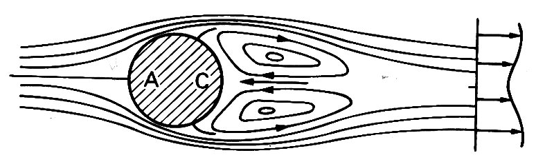
Fig. 5.22. Diagram showing the recirculating eddies behind a circular cyclinder, and a velocity profile across the viscous wake downstream. A and C are stagnation points.
Fluid elements are trapped there, circulating round and round while the main flow goes by. The motion in these vortices, where fluid velocities are significantly lower than in the main stream, is driven by the viscous stresses exerted by the main stream at the edges of the vortices. As Re increases (in the range 10-50) the vortices are progressively stretched out downstream.
Beyond the point where the main stream comes together again, there is a long, fairly narrow region where the velocity of the fluid is still less than that outside it in the undisturbed parts of the flow (a typical velocity profile is shown in Fig. 5.22). This region is known as the viscous wake of the body. Viscous wakes occur whether or not the fluid has a free surface, but are normally observable only at a free surface, where, however, they are often obscured by wave motions. For example, the wake of a ship is visible primarily because of the waves it generates on the sea surface, although this surface is also churned up by vigorous disturbances, partly induced by the propellers, which persist far downstream in a zone analogous to a viscous wake. When the stream of a river flows past the pier of a bridge, waves are of course generated, but, in addition, objects floating in the water can be seen to move more slowly behind the pier than in the main stream. Another familiar example of a wake occurs behind a rapidly moving lorry, where the forward motion in the wake (associated with the low pressure region immediately behind) tends to pull any small vehicle along with it. The backward motion at the sides of the lorry felt by anyone standing at the roadside (the slipstream) is a reflection of the increased relative velocity at the sides of a body (cf. Fig. 5.18 or 5.19). Of course, the Reynolds number in each of these examples is enormous (about 5 x 10⁶ either for a pier of width 2 m in a river flowing slowly at 2.5 m s-1 or for a lorry of width 4 m travelling at 15 m s~1 (just over 30 miles per hour)), but the gross features of the flows just described are always present.
At values of Re above about 40, the symmetrical steady flow depicted in Fig. 5.22 becomes unstable, and the wake is observed to oscillate slowly, with an amplitude which increases with distance downstream (Fig. 5.23).
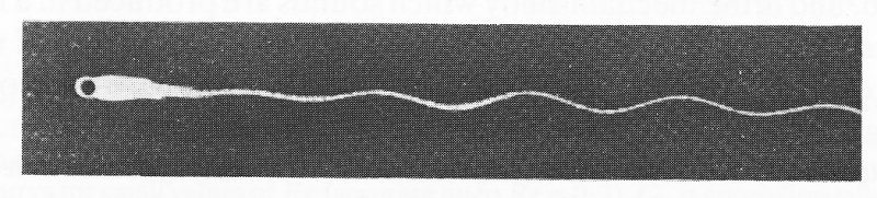
Fig. 5.23. Photograph of oscillations starting in the wake of a cylinder (Re = 55). (From Batchelor (1967). An introduction to fluid dynamics, P..2. Cambridge University Press.)
As Re increases further, the oscillation of the wake moves closer to the cylinder, and, when Re is near 60, begins to affect the two eddies behind the cylinder. They oscillate together from side to side, and appear to shed a small eddy at the end of every half-period, on each side of the cylinder alternatively. The behaviour of the wake at this stage is very striking (Fig. 5.24).
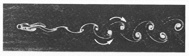
Fig. 5.24. Photograph of a vortex street (Re = 102), with arrows superimposed to show the direction of rotation of the vortices. (From Batchelor (1967). An introduction to fluid dynamics, Pl.2. Cambridge University Press.)
The fluid passing close to the cylinder gathers itself into discrete whirls, or vortices, arranged in two regular staggered rows, one on each side of the centre line. They are shown by the arrows in Fig. 5.24. This arrangement, called a vortex street, travels down-stream at a velocity less than U, and persists for very many cylinder diameters. This periodic pattern of the wake occurs also for a very wide range of Reynolds numbers up to about 2500. For still larger Re the wake is turbulent, and the discrete vortices cannot be easily identified, but even so the underlying periodic structure persists up to extremely large values of Re (at least 105).
Associated with the periodic vortex shedding there is a fluctuating pressure field in the neighbourhood of the body. This exerts a fluctuating force on the body, which may cause it to vibrate at the frequency of the vortex shedding if it is not rigidly fixed. These vibrations may in turn accentuate the intensity of the fluid mechanical oscillations, and so on. If the frequency of these oscillations is one at which the body can naturally vibrate with only a small stimulus, a potentially dangerous resonance may result (see Chapter 8, §8.4), in which the body oscillates more and more vigorously. Such resonance has been the cause of a number of engineering disasters, in which buildings have collapsed in a wind (a famous example is the Takoma Straits bridge, near Seattle, U.S.A., which collapsed soon after being built, in 1940). On a smaller scale, the periodic shedding of vortices is responsible for the humming of telephone wires in the wind, and is the mechanism by which sounds are produced in a number of musical instruments, particularly the human voice. The shedding of vortices in blood by obstacles such as the aortic valve or a stenosis will also generate fluctuating pressures which may be important (see Chapter 12).
The frequency f with which vortices are shed behind a cylinder can be related only to the parameters which determine the flow pattern: that is, the velocity U, diameter d, viscosity m, and density r. A simple quantity with the dimensions of frequency which can be derived from these is U/d, although more complicated quantities can be constructed by multiplying this by anything else which depends only on the dimensionless Reynolds number (Re = rUd/m). We may conclude, however, that the dimensionless quantity fd/U can depend only on Re, for a given shape of body. In fact this quantity, called the Strouhal Number, is approximately constant (0.2 for a circular cylinder) for a wide range of Reynolds numbers, above approximately 103, the Strouhal number is effectively constant. Over this range, the frequency of vortex shedding from a given body, and hence the pitch of the sound produced, increases in proportion with the flow velocity. The noise of the wind becomes more highly pitched as its speed increases.
The drag force exerted by a fluid flowing past a body, such as a circular cylinder, can be measured experimentally. In order to obtain a formula which can be applied to cylinders of different diameter in flows of different speed, we usually divide the drag by a quantity which also has the dimensions of force, and which can be thought of as a scale for a typical dynamic pressure force acting on the body. This quantity is
![]() (5.15)
(5.15)
where L is the length of the cylinder being used, which has to be very long for the flow to be approximately two-dimensional. The ratio of the total drag force to this quantity is called the drag coefficient, and is given by
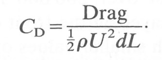 (5.16)
For cylinder cross-sections other than circular, the drag coefficient is similarly denned, only then the 'diameter' d has to be taken to be the maximum width of the cylinder in a direction at right angles to the oncoming flow (Fig. 5.25 (a)).
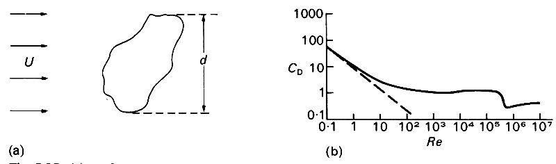
Fig. 5.25. (a) Definition of the diameter d of a cylinder of non-circular cross-section, for use in Equation (5.16), which determines the drag coefficient CD. (b) Graph of CD against Re for a circulary cylinder (logarithmic scales). The broken curve is the theoretical curve for small values of Re (accurate up to Re = 0.2). CD is approximately constant for values of Re between 200 and 200,000. (After Fox and McDonald (1973). Introduction to fluid mechanics, p. 408. John Wiley, New York.)
For any given shape of cylinder, the drag coefficient, like the Strouhal number, can depend only on Re. The relationship between CD and Re for a circular cylinder is plotted on logarithmic scales in Fig. 5.25 (b).
For very small values of Re, CD falls rapidly as Re increases. This is because, in that range, inertia forces are negligible compared with viscous forces, so that the 'typical' inertial or dynamic pressure force with which we have made the drag dimensionless in Equation (5.16) is not typical of the motion at all. In this case there is a balance between viscous and pressure forces; no boundary layer can be identified, since the presence of the body distorts the free stream equally in all directions. In fact, the streamlines approximately show fore and aft symmetry, just as in an inviscid fluid. Of course, the low Reynolds number flow is not similarly associated with zero drag, but, as we see from Fig. 5.25 (b), with a very large, viscous drag. The details of the flow at low Reynolds number can be analysed theoretically, on the assumption that the inertia is very small, and results in a prediction of the drag coefficient which is plotted as the broken curve in Fig. 5.25 (b). It can be seen to be accurate for values of Re less than 0.2.
We can also see from Fig. 5.25 (b) that for values of Re between about 200 and about 200 000 the value of CD is remarkably constant, at a value of about 1.2. This shows that the dynamic pressure force (Formula (5.15)) is certainly 'typical' of the flow. It reinforces the above statement that it is the change in the pressure distribution resulting from boundary layer separation which has the greatest influence on drag; the direct viscous drag is very small. The sudden fall in CD at a value of Re just over 200,000 is associated with turbulence developing in the boundary layer on the front of the cylinder (the wake will have been turbulent for much smaller values of Re). Rather than increasing the drag, as we might have supposed because of the increased viscous dissipation inevitable in a turbulent flow, it causes it to fall. The reason for this is that turbulence in the boundary layer inhibits boundary layer separation, by some mechanism as yet unknown. It causes the point on the cylinder surface at which the boundary layer separates to move towards the back (Fig. 5.26),
Fig. 5.26. Diagram indicating the extent to which turbulence in the boundary layer inhibits boundary layer separation, thus reducing the drag on the body.
which has the effect of reducing the area over which the reduced pressure in the separated region can act, so that the net difference in the pressure force between front and back must fall. Fascinating though this aspect of fluid dynamics is we shall not discuss it further since it cannot be relevant to the circulation, where the maximum Reynolds number for pipe flow is less than about 10,000.
We have concentrated so far on two-dimensional bodies because the flow patterns past them are easy to visualise. However, in many everyday examples of flow past bodies the body, and the flow round it, is three-dimensional. In fact the main features of the flow past three-dimensional bodies are similar to those already described, but it is important to recognise the few differences. The three-dimensional body most commonly studied is the sphere; this is because the flow past it is both more convenient to produce experimentally and more tractable to analyse theoretically than any other. Furthermore, many everyday examples of approximately spherical bodies come to mind: a large balloon rising through the air (large Re), a small grain of sand settling in water (small Re), a ball-bearing in oil (small Re), a ball in air (quite large Re), etc. In this case, the Reynolds number is again defined in terms of its diameter d and velocity U relative to the fluid far away, together with the kinematic viscosity (n) (i.e. Re = Ud/n). The drag coefficient is again the total drag divided by a typical dynamic pressure force, which for a three-dimensional body is usually taken to be 1/2rU2 times the area presented to the flow (1/4pd2 in the case of a sphere). Thus:
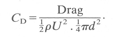
The graph of CD against Re is shown in Fig. 5.27, and can be seen to have a shape similar to that for a cylinder. Theoretical analysis at low values of Re shows that
![]()
and the curve corresponding to that is also drawn in Fig. 5.27.
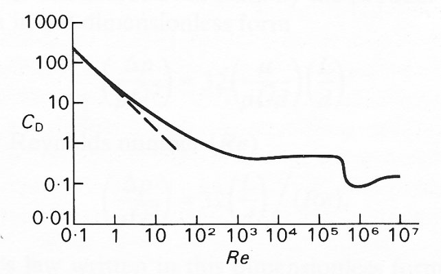
Fig. 5.27. Graph of CD against Re for a sphere; it is qualitatively similar to that for a cylinder. The broken curve is again the theoretical result for small values of Re. (After Fox and McDonald (1973). Introduction to fluid mechanics, p. 406. John Wiley, New York.)
The fixed eddies which form behind the sphere at higher Reynolds numbers, up to about 130, are of course not like the long straight vortices formed parallel to a cylinder. They are instead ring-shaped, since the overall motion is symmetric about an axis which passes through the centre of the sphere in the direction of the oncoming flow. (A more familiar example of a ring-vortex is given by a smoke ring, in which particles can be seen to rotate about a ring-shaped core as it advances.) At still higher Reynolds numbers, the ring-vortices are shed and create a complicated flow pattern in the wake. This is not an ordered motion like a two-dimensional vortex street, because the vortex remains a continuous closed loop, which becomes very distorted because of its tendency to be shed from different parts of the sphere at different times. Despite the apparent confusion in the flow behind the sphere, the perturbations in the force exerted by the fluid on the sphere are dominated by oscillations of a given frequency, leading to possible sound and vibrations at that frequency.