The mammalian heart consists of two pumps, connected to each other in series, so that the output from each is eventually applied as the input to the other. Since they are developed, embryologically, by differentiation of a single structure, it is not surprising that the pumps are intimately connected anatomically, and that they share a number of features. These include a single excitation mechanism, so that they act almost synchronously; a unique type of muscle, cardiac muscle, which has an anatomical structure similar to skeletal muscle, but some important functional differences; and a similar arrangement of chambers and one-way valves. Not surprisingly, the assumption has often been made that the function of the two pumps will also be similar. Thus it has become common practice to examine the properties of one pump, usually the left, and to assume that the results apply to the other also. This may often be unjustified, particularly in studies of cardiac mechanics, with the result that our knowledge of the mechanics of the right heart and the pulmonary circulation remains very incomplete. It must also be remembered that the scope for experiments on the human heart is very limited, and we must rely heavily on experimental information from animal studies. Thus the descriptions which follow apply primarily to the dog heart.
Many factors which affect the performance of the heart are not our concern in this chapter, among the most important being the wide range of reflexes which act on the heart. For example, nerve-endings in the aortic wall and carotid sinus are sensitive to stretch, and thus to changes in arterial pressure. A fall in arterial pressure, however caused, will reduce their frequency of initiation of nerve-impulses. This change, transmitted through nerves to the brain, alters activity in nerves passing to the heart, causing an increase in its rate and force of contraction. This in turn increases cardiac output and tends to restore the aortic pressure. A number of such reflexes, and a range of hormones reaching the heart via the bloodstream, are continuously modifying its performance in the intact animal, but since they are active physiological mechanisms, with origins outside the heart, we ignore them in this chapter. Thus no attempt is being made to provide a comprehensive description of normal cardiac function; only the muscular and mechanical features of cardiac pumping are explored.
The two pumps which make up the heart must operate over a wide range and be extremely well matched. Cardiac output in man may increase from a resting level of about 5 1 min-1 to 25 1 min-1 on strenuous exertion, and since we know that the ability of the pulmonary circulation to alter its volume (normally 0.5 - 1 l) is rather limited, the output of the two pumps must be the same except in the very short term.
The response of the heart in exercise involves an increase in rate of contraction and in output per beat (stroke volume). Thus the muscle fibres in the heart wall appear capable of varying both the time-course and the amplitude of their contraction, and it follows that the intrinsic contractile properties of cardiac muscle are of fundamental importance in any study of cardiac mechanics. They have, in the last twenty years, been the subject of intensive study, which was stimulated by the success of previous work on skeletal muscle in quantitatively describing the mechanical features of contraction. It has become clear that profound differences in functional properties exist which complicate the study (and the behaviour) of cardiac muscle, and different experimental methods and terminologies have added to the difficulties. Many interesting problems have emerged in translating the tension-generating and shortening properties of experimentally isolated slips of muscle into the pressure-generating and volume-ejecting properties of the intact ventricle, because the structure and geometry of the ventricle are complicated. Uncertainty about internal energy-losses in the muscle and the ordering and synchronicity of activation adds further difficulty here.
At the moment, therefore, although detail of the ultrastructure of the contractile apparatus is becoming available, our understanding of myocardial mechanics remains incomplete. The behaviour of the muscle is still described in terms of crude functional models, and the behaviour of the contracting heart-chamber can only be described qualitatively because of the geometrical uncertainties, even though the time-course and magnitude of the fluid-dynamic events in the cardiac cycle are being measured with increasing precision in both animals and man.
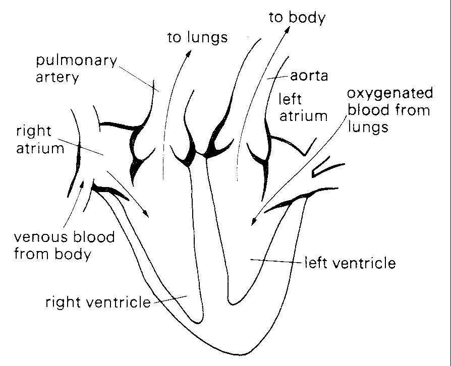
Each of the cardiac pumps consists of a low-pressure chamber (atrium), which is filled from a vein system and empties via a non-return valve into a high-pressure chamber (ventricle). The ventricle in turn passes blood on through a second non-return valve to an arterial system (Fig. 11.1).
Fig. 11.1. Diagrammatic representation of anatomy and directions of blood flow in the heart. septum. The veins draining into them communicate with them without valves.
The right heart receives blood from the body tissues via the systemic veins and pumps it into the pulmonary (lung) arteries. The left heart receives this blood from the pulmonary veins and pumps it into the systemic (main body) arterial circulation, via the aorta and its branches.
The two atria are comparable in structure; their walls are thin and relatively compliant, and they are separated from each other by a common wall, the atrial septum. The veins draining into them communicate with them without valves. The valves separating the atria from the ventricles (atrioventricular valves) differ slightly in structure on the two sides of the heart, the one on the right (tricuspid) having three cusps, the one on the left (mitral) two. These cusps consist of flaps, attached along one edge to a fibrous ring within the wall of the heart, and with free edges projecting into the heart-cavity. They are extremely thin (about 0.1 mm) and are made up largely of a meshwork of collagen and elastin fibres, covered by a layer of cells similar to those lining the walls of the heart-chambers and blood-vessels (the endothelium). The free edges of the cusps of both the mitral and tricuspid valves are 'tethered' to the wall of the respective ventricle by fine fibrous bands (chordae tendinae) which connect with slips of muscle (papillary muscles} projecting from the wall of the ventricle. Each chorda connects to the free edges of two cusps where they come in contact with each other when the valve closes; thus tension in the chorda generated by contraction of the papillary muscle at the beginning of systole counteracts the tendency of the increase in intraventricular pressure to turn the valve inside out and allow leakback into the atrium. There appears to be a self-contained mechanism for closure of these valves (see §11.5.1) in the flow events in late systole.
The exit valves from the ventricles (pulmonary and aortic) are very similar to each other, each consisting of three cusps with free margins reaching to the wall of the valve-ring. This arrangement allows opening to the full cross-sectional area of the valve-ring without distortion of the cusps. These cusps are not tethered, but can nonetheless support considerable pressure differences (in the case of the aortic valve, approximately 1.3 x 10⁴ N m-2 (100 mm Hg)). They are also extremely efficient, since only trivial backflow occurs through them during closure (which occurs more than 30 million times a year). Not surprisingly, their behaviour has been a source of interest for many years; in the fifteenth century Leonardo da Vinci examined their structure and made speculative drawings of flow patterns through them which have since proved remarkably realistic; their mechanism of action has recently been studied in detail (see §11.5.2).
The four valve orifices in the heart are aligned approximately in a single plane, and the cusps of each are attached at their bases to a stiff ring of fibrous tissue (Fig. 11.2).
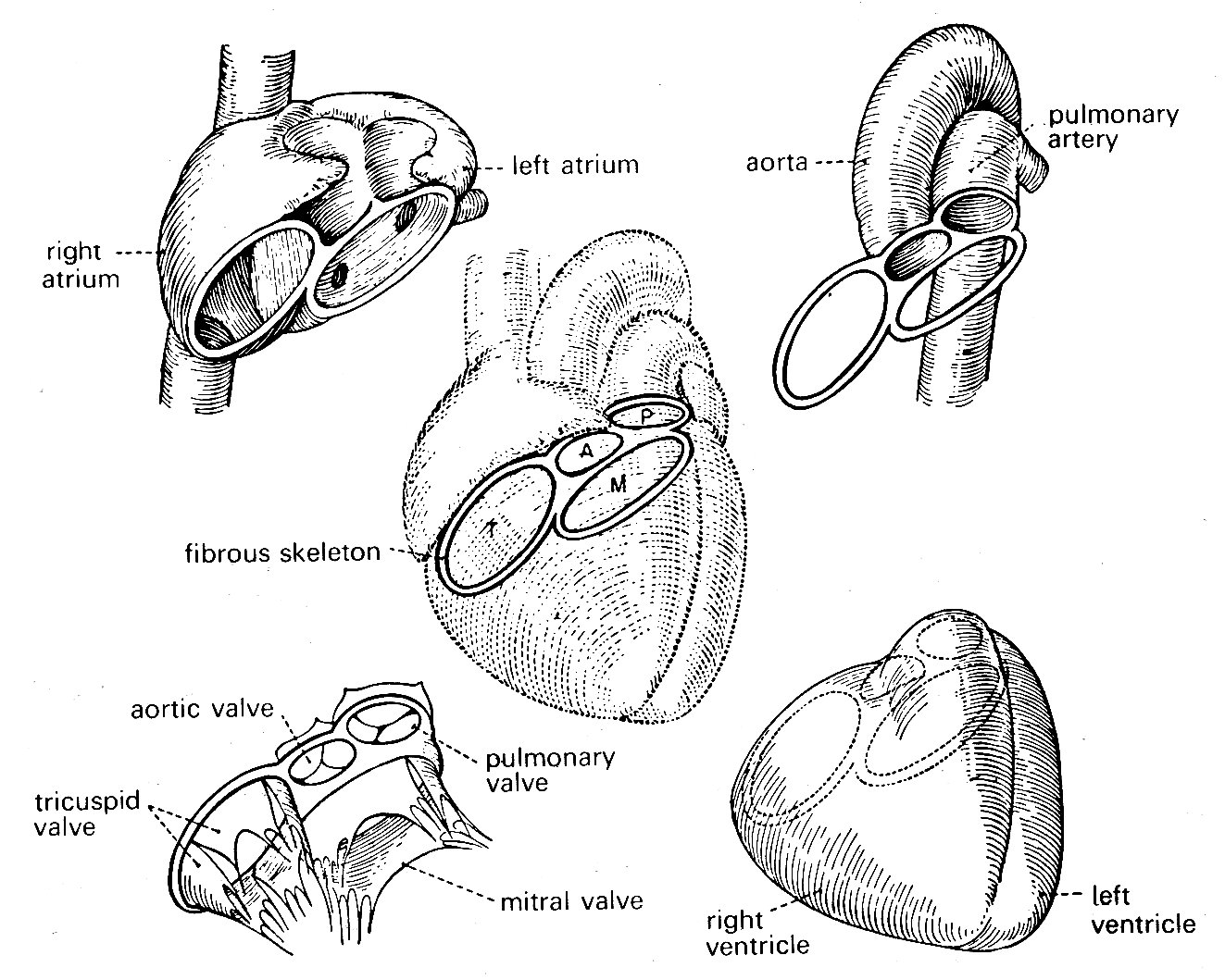
Fig. 11.2. Relationships of various structures in the heart. The 'skeleton' of the heart, consisting mainly of the fibrous valve-rings, also supports both atria and ventricles, and the two great arteries. (From Rushmer (1970). Cardiovascular dynamics. W. B. Saunders Company, Philadelphia.)
The four rings are in turn connected to each other by fibrous tissue so that the valve apparatuses are set in a stiff framework to which the muscle-fibres of each chamber are attached—the atria on one side, the ventricles on the other; and the pulmonary artery and aorta also attach at their origins to this plane of fibrous tissue. The whole heart is contained in a thin fibrous tissue bag, the pericardium, which in turn is attached to other structures within the chest, and through these to the vertebral column. The stress-strain relationship of the pericardium is, as can be inferred from Fig. 11.3, highly non-linear (Fig. 11.3).
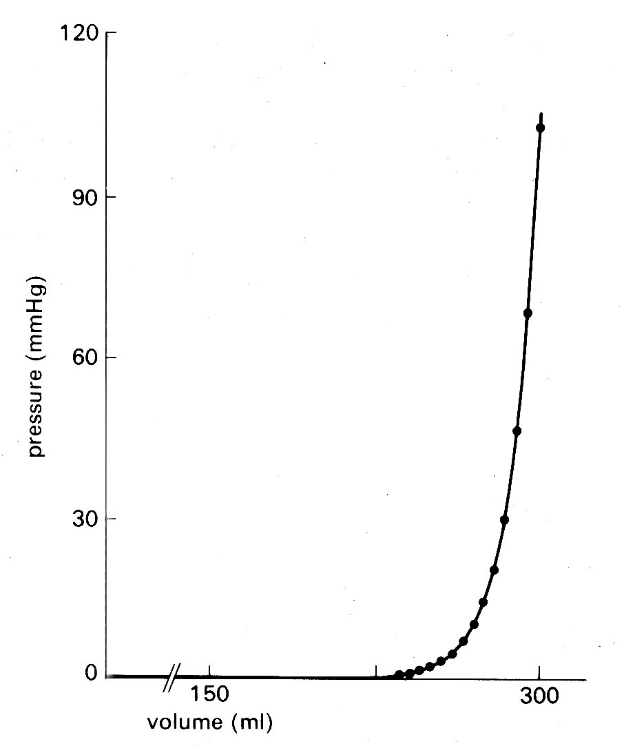
Fig. 11.3. Pressure-volume curve of pericardium of dog. (From Holt (1971). Circulation Res. 8, 1171. By permission of the American Heart Association, Inc.)
At normal diastolic heart volumes, the pericardium is only slightly stretched, and probably does not appreciably affect cardiac filling; in certain diseases where fluid accumulates within the pericardium, its constraint can restrict diastolic filling of the ventricles and severely reduce cardiac output (see §14.5.3).
The left ventricle is the only chamber whose wall-structure has been examined systematically. Recent studies of microscopic sections taken serially through the whole thickness of the wall have shown that older concepts of a ventricular wall made up of clearly defined muscle layers are incorrect, and that there is a well-ordered continuous distribution of fibre-orientation (Fig. 11.4).
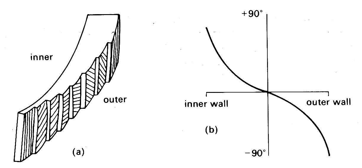
Fig. 11.4. Muscle fibre orientation in wall of left ventricle, (a) The orientation of the long axis of the fibres at successive depths from the outer surface, (b) The way in which the angle made by the fibre with the circumferential plane of the LV changes continuously through the wall (after Streeter et al. (1969), Circulation Res. 24, 339).
The innermost (endocardial) fibres run predominantly longitudinally from the fibrous region around the valves (the base) to the other end of the roughly elliptical chamber (the apex); the fibres slightly further out into the wall lie at a slight angle to the axis of the chamber, so that the fibres spiral slightly as they run towards the apex. This angulation increases in successively deeper fibres so that those approximately half-way through the wall run parallel to the shorter axis of the chamber, i.e. circumferentially; thereafter the angulation continues, so that the fibres at the outside (epicardial) surface are once again longitudinal. This arrangement gives the ventricle great strength even though individual muscle fibres can only bear tension axially, since a stress applied to the wall in outer wall any direction can be resisted by at least a proportion of the muscle fibres, and there is no direction or plane of weakness. Note that fibres do not have to terminate at the apex; they can turn and spiral back towards the base like string wound spirally on a stick. As can be inferred from Fig. 11.4 (b), there is a great preponderance of fibres with a circumferential distribution.
11.2.1 Electrical events. The contraction cycle of the heart is initiated in a localized area of nervous tissue in the wall of the right atrium known as the pacemaker or sino-atrial node. This has the inherent property of cyclical depolarization and repolarization (the latter process being dependent upon metabolic energy, derived ultimately from metabolism within the cells). When depolarization occurs in the pacemaker, it spreads at about 1 m s-1 into and through the surrounding muscle of the right and left atrial walls (causing atrial contraction) and then into a discrete nervous pathway (the atrio-ventricular bundle, or bundle of His) which passes through the fibrous tissue around the tricuspid valve ring into the muscular septum between the two ventricles; here it divides, and spreads into the muscle mass of each ventricle, terminating in a series of fine fibres amongst the muscle-cells (Purkinje fibres). The wave of depolarization spreads through this system rapidly (5 m s-1), and therefore depolarization and contraction of all the muscle-fibres in both right and left ventricles are relatively synchronous; the ventricular depolarization potential on the electrocardiogram—the 'QRS' component—lasts less than 0.1 s. A number of nervous and hormonal influences which originate outside the heart may act on the pacemaker to cause alterations of frequency, and may modify the conduction velocity of the depolarization wave through the heart; but the orderly sequence of atrial and ventricular contraction which follows pacemaker depolarization is ensured largely by the layout of the conducting pathways.
The cycles of depolarization and repolarization which occur in cardiac muscle generate small electrical potentials, and with suitably located electrodes these Can be picked up at the surface of the body, and amplified and recorded as the electrocardiogram. A typical tracing is shown at the top of Fig. 11.5.
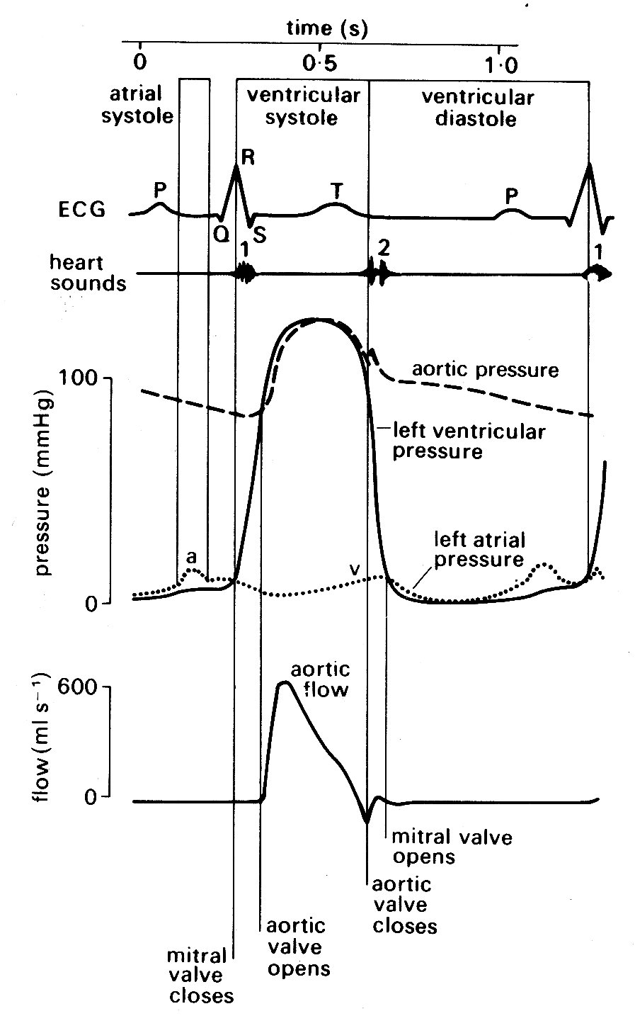
Fig. 11.5. Semi-diagrammatic illustration of the events on the left side of the heart during the cardiac cycle. All pressures related to atmospheric. The origin of the 'a' and 'v' wave in atrial pressure is discussed in the text, §11.2.2.
Depolarization of the atria produces a small deflection known as the T' wave; this is followed after a delay of about 0.2 s by a larger voltage deflection, often multiphasic, known as the 'QRS complex'. This reflects depolarization of the two ventricles, and is followed by a final component, the T' wave, which is generated during repolarization of the ventricles. The time relationships between these summed electrical potentials and the mechanical events on the left side of the heart can be deduced from Fig. 11.5, which shows the pressure and flow events that take place at a number of locations in the left side of the heart during a complete cardiac cycle.
11.2.2 Mechanical events. As has just been mentioned, the onset of ventricular contraction (ventricular muscle depolarization) is signalled electrically by the QRS complex of the electrocardiogram. Both ventricles contract almost synchronously (see Fig. 11.6),
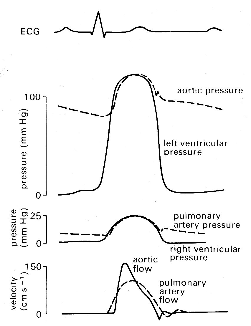
Fig. 11.6. Semi-diagrammatic illustration of pressure and flow occurring simultaneously on the left and right sides of the heart during the cardiac cycle.
but our description is simplified if we consider events on the left side of the heart only. The sequence of events is illustrated in Fig. 11.5. Depolarization is followed after a very short interval by the onset of active tension development (see §11.3.1) in the muscle fibres of the ventricular wall, and an increase in ventricular pressure. At this stage, the aortic valve is still held closed because the pressure in the aorta exceeds that in the left ventricle, and the cusps of the mitral valve are moving together as flow into the ventricle dwindles. Almost immediately, ventricular pressure rises above atrial pressure, and a brief period of backward flow from ventricle to atrium occurs, terminated by closure of the mitral valve. This is accompanied by a sound, audible at the chest wall and known clinically as the first heart sound. This marks the onset of systole, the period of ventricular contraction. The second heart sound marks the start of diastole, the period of ventricular dilatation. Note that these periods are defined in relation to the heart sounds and not in terms of muscle mechanics or the electrocardiogram.* [*Thus systole does not correspond exactly with the period of ventricular ejection, despite widespread use of the word in that sense.] In the ventricle, wall-tension now starts to rise extremely rapidly until the pressure within the cavity exceeds that in the aorta. There is no change in ventricular volume during this period, since blood is effectively incompressible; it is therefore known as the isovolumetric period. (In the older literature, it is often referred to as the isometric period; however, it is now clear that the ventricle does change shape during this phase, even though volume is constant, and the term isovolumic, or isovolumetric, is therefore preferable.) When the pressure within the ventricle exceeds aortic pressure, there is a net force operating to open the aortic valve, and the ejection phase of systole commences. The blood in the ventricle and proximal aorta undergoes rapid forward acceleration as left ventricular volume diminishes. Ventricular wall-tension then falls, the pressure difference between ventricle and aorta is reversed, and deceleration of aortic flow occurs. Finally, there is a brief period of backflow before aortic valve closure takes place, accompanied by the second heart sound. There then follows another isovolumetric period during which the muscle relaxes and ventricular pressure falls. At the same time, pressure in the left atrium is rising as it fills with blood from the pulmonary veins (the V wave). When its pressure exceeds that in the left ventricle, the mitral valve reopens. Ventricular filling then occurs, under the influence of a pressure difference generated at first passively and then by active shortening of the muscle fibres of the atrial wall; this active atrial contraction (atrial systole) is heralded electrically by the 'P' wave of the electrocardiogram, and marked mechanically by a brief increase in atrial pressure (the 'a' wave). Very shortly after this, activation of the ventricular muscle occurs and the cycle recommences.
In normal man, the heart-rate may range from about 45 min-1 (resting athlete) up to slightly above 200 min-1 on maximal exercise. Systole is much shorter than diastole at the lower heart-rates, occupying about a third of the cycle (Fig. 11.5); as the rate increases, there is a much greater shortening of diastole than of systole, until at the highest rates the two may be almost equal. The volume ejected from the ventricle with each beat (stroke volume) is normally in the range 70-100 cm3 at rest; a smaller volume remains in the ventricle - i.e. the ventricle ejects only 60-70 per cent of its contents. The variation in stroke volume with exercise is much less than that in the heart-rate; thus increases in cardiac output in severe exercise (five-fold or more) depend much more on rate increase than on stroke volume increase. Blood pressure rises in both the pulmonary artery and the aorta on exercise, but much more modestly than does the flow, because recruitment of additional vessels in the microcirculation, or dilatation of previously constricted ones, lowers the downstream resistance to flow.
11.3.1 Structure. Under the light microscope, the myocardium is seen to be made up of elongated muscle cells running in columns and having centrally placed nuclei and abundant mitochondria (Fig. 11.7).
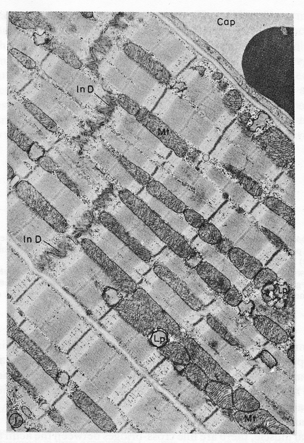
Fig. 11.7. Electron micrograph of parts of three cardiac muscle fibres and an adjacent capillary (Cap) in longitudinal section. The two upper cells are joined end to end by a typical steplike intercalated disc (In D). Rows of mitochondria (Mt) appear to divide the contractile substance into myofibril-like units but, unlike the true myofibrils of skeletal muscle, these branch and rejoin and are quite variable in width. Lipid droplets (Lp) somewhat distorted in specimen preparation are found between the ends of the mitochondria. xl5,000. The structure of a single sarcomere is shown at higher magnification in Fig. 11.8. (From Fawcett and McNutt (1969). 'The ultrastructure of the cat myocardium'. J. Cell Biol. 42, 1-45.)
As in skeletal muscle, the fibres have a cross-striated appearance which is due to the structure of the contractile units, or myoftbrils, lying within the cells. However, the motor nerve filaments, neuromuscular junctions, and the length-monitoring muscle-spindles present in skeletal muscle are absent from cardiac muscle; and further points of difference are that the muscle-cells branch repeatedly, and have abundant collagen fibres between them.
The limit of definition of the light microscope is about 0.25 mm, and at this level further detail is impossible to distinguish. Since there did not appear to be cell-membranes running across the fibres, it was assumed for some time that they had a syncytial structure, i.e. widespread continuity of cell cytoplasm. However, electron microscopy has revealed that the cell-membrane has two layers, with the inner layer passing across the fibres and dividing them every 50-100 mm into structurally separate cells, about 10-20 mm in diameter. At intervals of about 2 mm all along each such cell there are extremely fine invaginations of the cell-membrane known as T-tubules, which have been shown to provide for almost simultaneous activation of all the myofibrils in the cell when the membrane is depolarized.
Numerous other fine details of cell structure have been described, and a great deal of recent progress has been made in clarifying the biochemical reactions which release energy for contraction and repolarization. However, we will concentrate only on the contractile apparatus, since our interest lies in the mechanics of the muscle-fibres.
As mentioned previously, the contractile elements of each cell are the myofibrils, which run parallel to the long axis and show a repeating pattern of cross-striation. The myofibrils themselves actually consist of bundles of myofilaments, and the cross-striations repeat themselves because the myofilaments are made up of repeating chains of sarcomeres. The sarcomere is the fundamental contractile apparatus; its structure was first described in skeletal muscle, and has been confirmed in cardiac muscle with only minor differences. Each sarcomere is limited by two adjacent narrow bands known as Z bands or lines (Fig. 11.7); in between it is subdivided into a wide central A band, separated from each'Z band by a narrow, lighter I band. When the muscle-fibre is stretched, the distance between the Z bands widens; but the A bands remain the same length. All this can be distinguished under the light microscope; sarcomere-length increases with increase of overall muscle-length, and in heart muscle at its diastolic length is about 2.2 mm; the A band is 1.5 mm and the I bands 0.35 mm each.
A series of elegant electron microscopy studies has shown these bands to be due to partially overlapping parallel arrays of filaments, arranged as in Fig. 11.8.
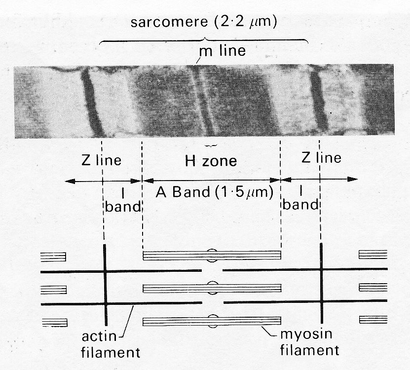
Fig. 11.8. Above: sarcomere structure as seen with the electron microscope. The sarcomere is bounded by a pair of Z bands. Within it is the dark central A band (marked at its midpoint by the darker m line) and two paler I bands.
Below: shows in schematic form the disposition of the rods of the contractile proteins actin and myosin which give rise to this appearance. Note that at this length the actin filaments do not reach past the midline of the sarcomere, so that no 'contraction band' is visible. See text for details. (From Sonnenblick, Spiro, and Spotnitz (1964). Am. Heart J. 68, 336.)
The thicker filaments making up the A bands are composed primarily of the protein myosin; the thinner rods which interdigitate with them are actin. When the muscle is stretched, the Z bands move apart and the actin rods slide along and partially disengage from the myosin rods; thus the I bands widen. When the muscle contracts, the reverse happens, until at very short muscle-lengths the I bands disappear, and new dark bands ('contraction bands') appear where the actin rod tips overlap each other at the centre of the A band. This occurs at sarcomere lengths less than 1.5 mm.
In skeletal muscle, there are fine cross-bridges between the actin and myosin filaments, projecting from each thick (myosin) filament. There is probably one cross-bridge per molecule, and they are spaced about 6 nm apart, arranged helically at 60° intervals round the myosin filament. Each myosin filament is surrounded by six actin filaments, and therefore makes one cross-bridge with each of these in a length of approximately 40 nm.
The cross-bridges seem likely to have an important role in the shortening process of striated muscle, since the filaments themselves are probably too far apart for direct interaction; one suggestion is that during contraction the cross-bridges may move back and forth, hooking up to specific sites on the actin filaments and drawing them on before releasing the linkage and moving back to a new linkage site. Thus during activity they would have a ratchet action; with the cessation of activity the filaments would be free to slide apart passively. To date, this remains a speculative explanation, particularly when applied to cardiac muscle.
11.3.2 Static mechanical properties of cardiac muscle. The 'sliding filament' description of sarcomere behaviour outlined above is doubly compelling because it not only fits with the visible ultra-structure of muscle, but offers an explanation of one of its fundamental mechanical properties - the length-tension relationship. When a muscle is held at a constant length and stimulated electrically it generates tension (active or developed tension) over and above any resting tension present prior to stimulation. If this experiment is repeated with successive small increments in length, the active tension is found to increase successively to a peak and then decline (Fig. 11.9).
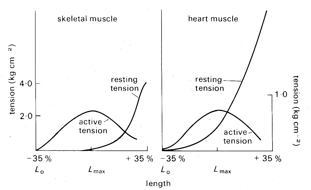
Fig. 11.9. Typical length-tension curves for skeletal and cardiac muscle. In each case resting and active tension was plotted against length as the muscle was held at a series of lengths and stimulated electrically to contract. The ordinates show tension, expressed in kilograms per square centimetre of muscle cross-sectional area. Note the difference in scaling of the two graphs. The abscissae show sarcomere lengths, relative to the lengths Lmax, at which the maximum active tension was developed; in these experiments Lmax was 2.2-2.3 mm for both skeletal and cardiac muscle. (After Spiro and Sonnenblick (1964). 'Comparison of the ultrastructural basis of the contractile process in heart and skeletal muscle'. Circulation Res. 15, supplement 2, pp. 14-37. By permission of the American Heart Association, Inc.)
This is true for a wide variety of muscle, and in skeletal muscle (and probably also cardiac muscle) the peak of the length-tension relation comes when the degree of stretch brings sarcomere length to about 2.2 mm. Fig. 11.9 suggests that in absolute terms (i.e. per unit cross-sectional area) heart muscle is much weaker than skeletal muscle. This may be more apparent than real, since heart muscle contains a greater bulk of non-contractile tissue such as collagen and mitochondria, and the muscle fibres are not all parallel. In muscle which has contracted at sarcomere lengths of less than 2.2 mm, the actin rods reach right in past the midpoint of the myosin rods and overlap their opposite numbers; it is postulated that this interferes with the formation of cross-linkages so that less than maximum tension can be developed. This overlap lessens as the muscle is stretched, until at a sarcomere length of 2.2 mm the actin and myosin rods cease to have a double overlap, and the maximum number of cross-linkages can be formed. It is at this length that the maximum active tension can be developed. As the sarcomere is stretched beyond this, the actin rods are progressively withdrawn from between the myosin rods, and fewer cross-linkages can form. In this length range, the active tension developed in a contraction declines linearly with length increase, until at a sarcomere length of about 3.5 mm the actin rods are fully withdrawn and the muscle ceases to generate any active tension.
In skeletal muscle this relationship between sarcomere length and tension has been firmly established, and its functional significance is generally agreed. The behaviour of sarcomeres in cardiac muscle has been investigated much less thoroughly; under physiological conditions they appear to operate in the length range from about l.5 mm to 2.2 mm - sarcomeres measure approximately 2.2 mm when ventricular diastolic pressure is about 12 mm Hg, which is the upper limit of normal, and thus the sliding filament hypothesis is an attractive explanation of myocardial length-tension relations. However, relatively few observations have been made on the relationship between sarcomere length and developed tension in cardiac muscle, and these are to some extent conflicting. This may be because of technical problems, particularly those of tissue distortion during histo logical preparation; methods have recently been developed to measure sarcomere length in vivo, and these may resolve the question. At present, it seems well established that no active tension is developed at sarcomere lengths less than about 1.5 mm and that the peak of the length-tension curve normally occurs somewhere between 2.0 mm and 2.2 mm, as it does in skeletal muscle. In between it is not clear whether increasing tension is the result of successive increments in sarcomere length as in skeletal muscle, or recruitment of increasing numbers of sarcomeres in muscle-fibres which were buckled at short muscle-lengths and are straightened and then stretched as the muscle lengthens. Furthermore, there is recent evidence that the curve relating tension and sarcomere length (Fig. 11.9) may be displaced along the sarcomere length axis in response to changes in the chemical environment of the muscle. We need a more detailed knowledge of the behaviour of actin-myosin cross-linkages to settle these uncertainties.
In skeletal muscle, the linear relationship between muscle-length and sarcomere length is maintained until the latter reaches at least 3.5 mn, and the progressive reduction in available cross-linkage sites as the actin and myosin filaments are gradually pulled apart offers an adequate explanation of the linear decline of active tension along the 'descending limb' of the length-tension curve. For heart muscle, the situation at high degrees of stretch is different. Sarcomeres will lengthen to only about 2.6 mm and even in this range the linear relationship described above does not hold; increments in overall muscle-length beyond this point require the imposition of very high resting tensions and probably involve sliding of whole fibres relative to each other. This situation does not arise in the normal heart and seems very unlikely even in the failing or pathological heart; in acute experiments where the relaxed left ventricle was distended with pressures as high as 100 mm Hg (far in excess of the levels reached even in severe heart disease) the sarcomeres in the ventricular wall had an average length of only 2.3 mm.
11.3.3 Dynamic mechanical properties of cardiac muscle. The length-tension curve describes an important property of muscle under static conditions - held at a constant length both before and during activity - but it throws no light on the dynamics of muscular contraction, which are of fundamental importance to any understanding of heart muscle performance.
A stimulated muscle goes through a period of mechanical activity (the 'active state') which reflects the release of energy derived from chemical reactions and has measurable properties both of duration and intensity. Enormous progress has been made in elucidating and measuring both the biochemical steps which yield energy, and the mechanical behaviour which is the expression of this energy release. The literature is voluminous, reflecting both the technical difficulties involved in research on the myocardium and its innate complexity, and the subject can only be briefly surveyed here.
The commonest material used for experimental study of the mechanical properties of heart muscle has been papillary muscle, removed from the right ventricles of young animals under anaesthesia. It can be obtained in this way as extremely thin strips a few millimetres in length, and made up of numbers of fairly parallel muscle fibres. When such papillary muscles are mounted in oxygenated, nutrient media of appropriate ionic and osmotic properties, they preserve their contractile properties in response to electrical stimulation for long periods. These contractile properties have been interpreted largely in terms of very simple mechanical models; to demonstrate why such models were chosen it is necessary briefly to describe some early experimental work carried out on skeletal muscle.
Intact skeletal muscles can be removed easily from small animals such as the frog, and a number of workers in the early years of the twentieth century studied these muscles, stimulating them electrically and examining the mechanical properties and heat production during contraction (the latter phenomenon having been demonstrated by Helmholtz over fifty years previously).
As was mentioned earlier, electrical stimulation of muscle leads to tension development. In the resting state, a potential difference of about 90 mV is maintained across the membrane of the muscle-cell - the resting potential. An externally applied shock can cause transient reversal of polarity of this potential, followed by slow recovery. This discharge, which is known as the action potential, triggers the release of calcium ions from stores within the muscle-cell, and these somehow activate the cross-linkages between the actin and myosin rods in the contractile apparatus of the sarcomeres. This whole process occurs within milliseconds, and the muscle cell is then capable of contracting (i.e. shortening and/or generating tension) for a short time before metabolic processes within the cell remove the calcium ions and the muscle returns to the resting state.
Thus a single electrical stimulus applied to a muscle-fibre causes a short-lived contraction appropriately known as a twitch. A chain of stimuli causes repetitive twitches, and in skeletal muscle if the stimulation frequency is high enough the twitches will fuse together to give a sustained contraction. This is known as a tetanus, and the corresponding train of shocks is a tetanic stimulus.
For a given muscle preparation, the tension generated in each twitch or tetanus will increase with increasing stimulus strength until a maximum is reached which is highly reproducible over long periods of time. If the muscle is held at constant length, the twitch or tetanus is known as isometric; if it is allowed to shorten, the force (if any) opposing shortening is described as the load (or afterload) and if this force is constant, which implies that all accelerations of the load are very small compared to that due to gravity, the contraction is called isotonic. Since maximal isometric contractions were found to be highly reproducible, they were used experimentally as the baseline condition; in this case the muscle generated heat during the course of a stimulation cycle, but since no shortening occurred, no external work was done (work, or energy, is equivalent to force times distance). When muscles were allowed to shorten by a distance x against a load or force P, not only were Px units of work done, but an extra amount of heat was released. (This effect of shortening on heat production is known as the 'Fenn effect' after its discoverer; Fenn (an American physiologist who did this work in 1923) also demonstrated the converse to be true - if a muscle was stretched during stimulation, it gave out less heat than when held at constant length. In describing this experiment, Fenn coined a phrase, 'negative work', which has given pain to physical scientists ever since; this is unfortunate, since the implication of the experiment - that the mechanical conditions during contraction control the amount of energy released - is fascinating and appears to have been little explored.)
The explanation of this liberation of excess heat on shortening came some years later when instruments capable of following heat-production instant by instant through the contraction and relaxation cycle became available. It was then shown in a famous series of experiments carried out by A. V. Hill that the extra heat associated with shortening is proportional to the distance x shortened; thus it is equivalent to ax units of work where the constant a has the dimensions of force. Now the amount of mechanical work done is Px units; so the total extra energy released in shortening is (P + a )x, and the rate of release of energy is (P + a) v, where v (= dx/dt) is the velocity of shortening. This rate of energy liberation was found experimentally to increase as load diminished, having its highest value when the load was zero and being zero when the muscle exerted its maximum force in an isometric contraction. The relationships were found experimentally to fit best in the form
(P + a) v = b (P0 - P), (11.1)
where b is a constant with the dimensions of velocity. This can be rewritten
(P + a)(v + b) = b (P0 + a), (11.2)
where the right-hand side is a constant and a hyperbolic relationship is predicted between the force P and velocity v of contraction. Thus the properties predicted from thermal measurements were open to confirmation by purely mechanical experiments, and were indeed verified when the velocity with which a muscle could shorten isotonically against various loads was examined (Fig. 11.10).
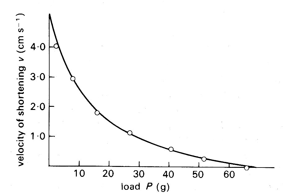
Fig. 11.10. Relationship between load P (grams-weight) and velocity of shortening v (cm s-1) in isotonic shortening of frog skeletal muscle. The points were obtained experimentally; the line was derived from Equation (11.2) in the text. (From Hill (1938). Proc. R. Soc. B 126, 136.)
The thermal observations were, however, of great importance in another way, since they suggested the first conceptual mechanical model of the muscle fibre. Observations on the course of heat release in the very early stages of stimulation revealed that it was similar for both isometric and isotonic contractions. This suggested that similar mechanical events were occurring in the early stages of both types of contraction, and since the length of the muscle fibre could not change in an isometric contraction, the idea arose of a contractile element in the muscle, which shortened on stimulation but which was linked in series to an elastic element that could lengthen if muscle length was held constant (Fig. 11.11 (a)).
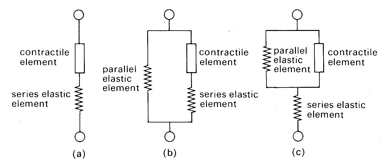
Fig. 11.11. Mechanical models of muscle.
The force-velocity relationship described above was assumed to describe the properties of the contractile element, since in steady shortening under isotonic conditions the elastic element would have constant length and would not contribute.
It should be stressed that Hill was examining the properties of skeletal muscle under very particular conditions. First, the muscle was stimulated with trains of high frequency shocks (tetani), so that a prolonged and maximal response occurred. Thus each observation was carried out with a constant load and a steady velocity of shortening. The real physical properties of the series elastic element were not considered, since it was at constant length throughout. Similarly, the time-course of development (or decay) of force was ignored. Furthermore, resting tension was very small at the muscle-lengths used (approximately 2 per cent of active tension), and therefore a model with two elements was adequate. The addition of a component to account for tension in the resting state (parallel elastic component, as in Fig. 11.11 (b) and (c)) which becomes necessary to allow for resting tension at longer muscle lengths (Fig. 11.9) was not considered in any detail; it was represented as a simple elastic element with no part to play in active shortening, and its nature and mode of coupling to the other two were deliberately left vague. Finally, the exact nature and location of the contractile element and the series elastic element also remained undefined; structures such as tendons might represent a genuine elastic element, or the internal contractile mechanisms might be elastic. Nonetheless, this 'two-element' model of active skeletal muscle achieved widespread acceptance, since it explained a range of mechanical and thermal observations. It was natural, in view of the structural similarity which exists between sarcomeres in cardiac and skeletal muscle, to consider its applicability also to cardiac muscle.
Problems arose immediately. First, cardiac muscle preparations exhibit appreciable tension throughout the range of lengths from which they will contract; thus the parallel elastic element becomes an essential part of the model, and the force-velocity relation can be examined only incompletely, since forces at and near zero cannot be achieved. Second, and far more important, is the fact that under normal conditions it is not possible to tetanize cardiac muscle like skeletal muscle and get a sustained and highly reproducible isometric contraction. Cardiac muscle repolarizes relatively slowly, and repeated stimuli do not produce a steady, maintained contraction. Instead, they produce twitches which even at high stimulation frequency only partially merge, giving a 'saw tooth' time-course of tension or shortening. Thus an incomplete cycle of relaxation and contraction occurs with each stimulus. At lower frequencies, stimuli evoke twitches which are clearly separated and may be highly reproducible, but neither of these types of response represents a steady state of activity, since the tension-generating and shortening capacity of the muscle (its active state) may be changing continuously during a contraction. A series of twitch responses from a papillary muscle preparation is shown in Fig. 11.12.
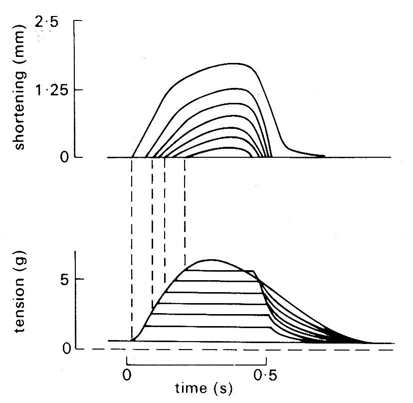
Fig. 11.12. A series of superimposed records showing the length and tension changes that occur in a cat papillary muscle which contracts against a series of different loads. The initial length was held constant; the lower family of curves shows that tension rose to match the load in each case, and then remained constant whilst shortening occurred. The amount of shortening at each load is shown in the upper curve. The final tension curve shows the response when the muscle cannot lift the load; this is the isometric twitch response. (From Sonnenblick (1962). Am. J. Physiol. 202, 931.)
This greatly complicates the design and interpretation of experiments. The intensity of the active state (however it may be assessed) is obviously an important property of the muscle; but it becomes extremely elusive if it is changing throughout a contraction. The problems are best illustrated by examples. Hill originally defined active state as the tension which the contractile element could bear without changing length; thus it could only be measured when the contractile element velocity was zero. Even in skeletal muscle this was only easy when tension had reached a sustained maximum value in an isometric tetanus; in this situation the contractile element has moved right along the force-velocity curve (Fig. 11.10), shortening progressively more slowly against the growing tension in the stretched series elastic element until it comes to rest; the intensity of the active state is then given by the value of P0 (Equation (11.1)). If on the other hand the contraction is not steady, but takes the form of an isometric twitch in which the active state rises and then falls, it is obviously extremely unlikely that the contractile element would be brought to rest by the load just at the time when activity was maximal. But unless this happens, the maximum recorded tension will not correspond to Po, and the intensity of the active state will be underestimated. The measurement is feasible if some means is devised to hold contractile element length constant, for example by controlled stretching of the muscle during the contraction; but the experimental difficulties are very great.
An alternative approach (which to some extent added confusion, since it introduced another definition of active state) has been to use the unloaded velocity of shortening as an index of active state. This is easier to examine experimentally; the muscle is released from its load at different points during successive twitch cycles and the velocity of shortening is measured immediately after the muscle has sprung back to unloaded length. An example of the results obtained in such an experiment is shown in Fig. 11.13;
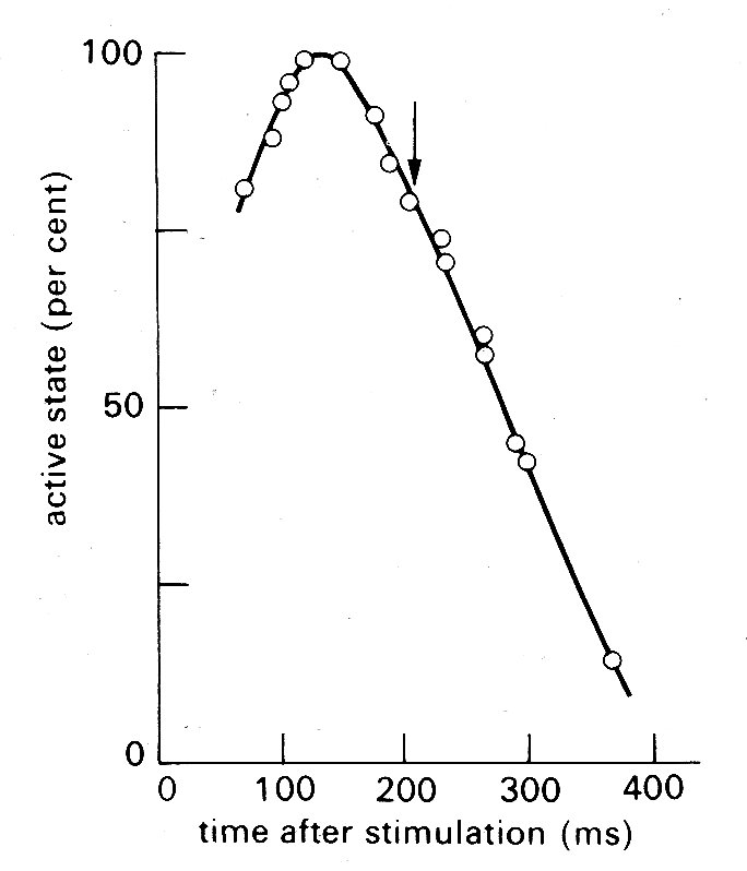
Fig. 11.13. Time-course of active state in cardiac muscle as measured by released isotonic contractions. The arrow shows the time at which peak tension was achieved in an isometric twitch. (From Edman and Nilsson (1968). Acta Physiol. Scand. 72, 205.)
the active state rises to a peak about 150 ms after stimulation (a little before peak tension is reached in an isometric twitch) and then declines steadily.
Recently, however, the techniques based on contractile element velocity have been shown to have a flaw because the duration of active state has been found to depend on length changes in the contractile element; if it shortens at any point in the contraction, the active state wanes earlier. In recent experiments, therefore, the subject has been re-examined by a more sophisticated approach; the stress-strain characteristics of the series elastic element in a muscle are measured first, and then computer-controlled mechanical feedback is used to pull on the muscle during contraction so that it is continuously lengthened by just the amount necessary to keep the contractile element length constant; the tension on the muscle at each instant through the contraction cycle then defines the active state. This method gives a time-course and intensity of active state which differ only a little from the isometric twitch response, the chief difference being a fractionally earlier rise and fall in active state. Even this, however, is unlikely to be the last word, because it has been demonstrated still more recently that the series elastic element has time-dependent properties, and the amount of stretch needed at different times in the cycle to fix contractile element length will therefore not depend solely on instantaneous tension.
These studies, culminating with the paradox that the contractility of a papillary muscle preparation is best defined by an experiment in which it is forced to lengthen, are described in some detail because they highlight the difficulties which arise in the experimental study of cardiac muscle mechanics at this level. It should by now be apparent that at least four variables - time, length, tension, and velocity - are important; and a whole range of extraneous factors which affect contractility such as temperature, oxygenation, and ionic environment need stringent control. Blinks and Jewell* have provided a useful recent survey of the subject; they point out that since the standard experiment explores the relationship between a pair of variables, six classes of experiment are needed to explore the inter-relationships between time, length, tension, and velocity. [* Blinks, J. R., and Jewell, B. R. (1972), "The meaning and measurement of myocardial contractility'. Chapter 7 in Cardiovascular fluid dynamics, ed. Bergel, D. H., Academic Press.] We do not explore this subject in detail, but certain general conclusions are important enough to need stating. The inverse relationship shown to hold for skeletal muscle between developed force and velocity of shortening (Fig. 11.10) applies also to cardiac muscle (though it is not usually precisely hyperbolic). This must be immediately qualified by pointing out that the force-velocity relationship is influenced by muscle-length and by the active state of the muscle. The effect of length can be predicted qualitatively from the length-tension relationship shown in Fig. 11.9; as the initial length increases, the force-velocity curve is shifted upwards on its axes. Thus in order to present the properties of the muscle graphically, we would need a three-dimensional plot, with two of the axes being contractile element force and velocity (as in Fig. 11.10) and the third being muscle-length. Then at any level of active state in the muscle, the various possible combinations of these would form a three-dimensional surface within the axes.
In practice, it is difficult to draw such graphs realistically, because they need to show both positive and negative velocities (i.e. shortening and lengthening), and the rising and falling limbs of the length-tension relationship, if they are to describe the whole contraction. In trying to understand how the properties of the muscle interact, it is easier just to consider two types of contraction - isometric and isotonic.
The simpler example is an isometric twitch, since it avoids muscle-length changes. The contraction starts at some point on the resting length-tension curve (Fig. 11.9). Initially, the contractile element begins to shorten very fast, since it is relatively lightly loaded; thus velocity rapidly increases. However, since shortening of the contractile element implies lengthening of the series elastic element, force builds up and the contractile element velocity is then reduced progressively until it becomes zero; at this point the maximum force (equal to the sum of active plus resting tension in Fig. 11.9) is being developed, and the muscle has moved along the force-velocity curve in Fig. 11.10 to intercept the load (force) axis. Thereafter, relaxation occurs, and the muscle returns to the original starting point on the resting length-force line.
If the muscle shortens against a load during contraction (isotonic contraction) the situation is slightly more complicated. At first the contractile element shortens and develops force, stretching the series element as for the isometric case. Then a point is reached where the force equals the load; thereafter, force remains constant, and the whole muscle begins to shorten with the series elastic element at constant length. The demand for constant force at diminishing muscle-length can only be met by a diminishing contractile element velocity (Fig. 11.14);
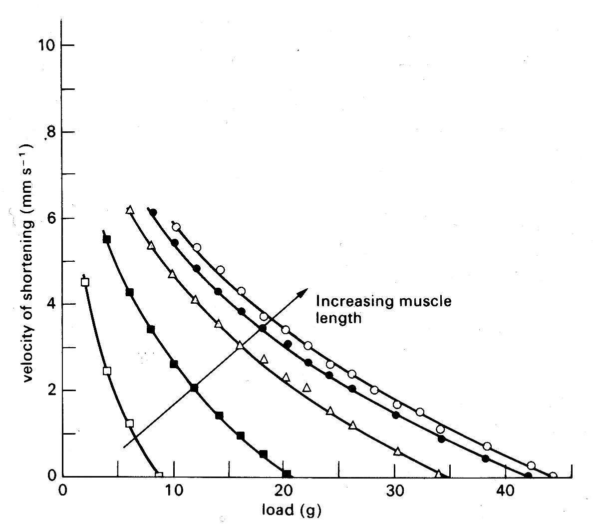
Fig. 11.14. Curves illustrating the length dependence of the force-velocity relationship in cardiac muscle. Each curve is plotted from a series of contractions against different loads such as those shown in Fig. 11.12. Successive increases in the initial length of the muscle displaced the curves farther and farther to the right. (After Sonnenblick (1962). Am. J. Physiol. 202, 931.)
so the muscle shortens more and more slowly, until it begins to relax, and again returns to the starting point on the resting length-tension curve.
In the real heart, both isometric and isotonic phases occur during contraction, and, as will be seen later, the load (i.e. force) is changing continuously during the isotonic phase; it is easy to imagine that the detailed behaviour during such a contraction would be extremely complicated. Furthermore, we have ignored a major factor which complicates all these relationships - the importance of time. Active state does not remain constant throughout the contraction, but waxes and wanes, so that the force-velocity curve, which has a shape like that in Fig. 11.10, represents properties at only one instant; it has grown from the origin following stimulation of the muscle, and will collapse back into it as the active state decays. The graphs relating force, velocity, and length are all moving with respect to their axes during the contraction and relaxation of the muscle.
This kind of description has some value both in illustrating the complications that exist and in showing that however we examine a contraction (whether in terms of velocity or force) there are two main influences at work in deciding its level. The first is the length of the muscle element, and the second is the intensity of the active state. The importance of this latter property is worth stressing; it is easy to see intuitively that a high level of active state will, other things being equal, produce a stronger contraction - however measured. But it is much less easy to see how to express or measure this level, and in many situations we find that there is a property of the muscle—usually termed 'contractility' - which is not precisely measurable or definable. Even if we confine attention to the isolated muscle preparation there are a number of areas still in dispute. These are mainly related to the form of the 'edges' of the three-dimensional surface which is needed to describe graphically the inter-relations between force, velocity, and length described above, which cannot always be described directly from experimental evidence, but only by extrapolation. Such extrapolation must be based on a model of the muscle (such as Fig. 11.11 (b) or (c), or some more complicated variant) and the result may be crucially dependent upon which model is chosen.
One example, which has important practical implications, will serve to illustrate the problem. It concerns the maximum velocity of shortening which can be achieved by the unloaded contractile element. This velocity (known as Vmax) cannot be measured directly in cardiac muscle because, as shown in Fig. 11.9, there is finite tension at all lengths in resting cardiac muscle, and therefore there has always to be a load (the preload) present to set the initial length. Thus Vmm can only be established by extrapolation. Some years ago, the American physiologist E. H. Sonnenblick performed this extrapolation on force-velocity curves measured at a series of different muscle-lengths, and concluded that it was possible to extrapolate all the curves (which are shown in Fig. 11.14) to a common intercept on the velocity axis.
Thus Vmax appeared to be independent of muscle-length. This suggestion stimulated great interest because it implied that Vmax might be used to distinguish between the effects which changes in length and in active state intensity (i.e. contractility) have on muscle performance. It will already be clear how useful such a measure would be in isolated muscle experiments; but in examining the performance of the whole heart chamber, where the difficulties of controlling and monitoring these separate influences increase, it would be even more valuable.
However, there are problems in performing the extrapolation which gives Vmnx, because some shape has to be assumed for the force-velocity curve which is being extrapolated, and it is in choosing this that the muscle model becomes important. Now Hill's model of muscle (Fig. 11.11 (a)) is inappropriate, because in the heart there is resting tension, so it becomes necessary to correct the measured data, to allow for the effect of a parallel elastic element, before extrapolating. The details of this can be found elsewhere;* [* Pollack, G. H. (1970). 'Maximum velocity as an index of contractility in cardiac muscle', Circulation Research, 26, 111-27.] it suffices here to say that the corrections needed depend upon which form of model is used (Fig. 11.11 (b) or (c)) being the simplest possibilities), and affect the values derived for Vmsa. This means that the original hypothesis that Vmax was independent of initial length, which was based on extrapolation of the curves in Fig. 11.14 to a common origin on the velocity axis, may be true only as a special case, and the length-velocity relationship at zero load has once more become a subject of dispute. During the decade or so in which these simple mechanical models have been used in cardiac research, much of the detailed ultrastructure of skeletal muscle has been described, and elegant techniques developed for making measurements at the sarcomere level. Increasingly, the mechanical properties of skeletal muscle are being interpreted in relation to the known structure of the contractile apparatus; thus the sarcomere has become the model. So far, a lack of suitable preparations has prevented this in cardiac muscle research, and the mechanical models continue to be the only useful analogy to real cardiac muscle at present.
11.3.4 Summary. Before we go on to consider the behaviour of the intact heart-chamber, it is useful to summarize some of the findings on isolated muscle preparations. Such muscles contain considerable numbers of muscle-cells, probably all lying reasonably parallel with the long axis. At rest, and over what can be assumed to be their normal operational length range, they resist stretching with a force which rises steeply with increasing length. The structural element responsible for this property has not been identified; in conceptual models it is called the parallel elastic element, and thought of as a spring (though a simple spring is actually a poor representation of the real situation, since the muscle does not oscillate when it is released, and exhibits a good deal of creep when it is stretched; both these imply viscous as well as elastic properties). Cardiac muscle-cells can be depolarized by an externally applied shock, and this depolarization is followed, after a delay of some milliseconds, by a period of mechanical activity during which the muscle will shorten. If it is loaded to resist shortening then it develops tension, and shortens if and when tension matches the load; the velocity of shortening is then inversely related to the load moved. The ability of the muscle to pull and shorten undoubtedly resides in the structures in the sarcomere, whose length is closely proportional to muscle-length over a considerable range. However, the details of the shortening mechanism are unresolved, so again a conceptual model is used, comprising the contractile element, which shortens on stimulation, and is connected to the load (if any) via a series elastic element. The magnitude of force and velocity generated by the muscle increases, in the physiological range, with muscle-length; thus a family of force-velocity curves are needed to describe contractions starting from different lengths. Beyond a certain length, which probably corresponds to some optimal alignment of the protein filaments in the sarcomere, further stretching produces a decline in the force generated by a contraction; but this probably lies outside the normal range of lengths in the intact heart. The individual sarcomere will apparently shorten by a maximum of about 30 per cent, from a resting length of approximately 2-2 mm down to 1-5 mm; but such measurements may be imprecise due to distortion during histological preparation. The time-course of contractility of the muscle is limited, as is its intensity. For practical purposes, these limits are probably well described by the isometric twitch response, and both are susceptible to a number of environmental influences. Influences which affect the time-course of cardiac contraction (i.e. heart-rate) are known as chronotropic; and those which affect its magnitude as inotropic. Inotropic influences include a number of chemical agents, such as hormones, drugs, and ions, which may increase or decrease the contractility and are likely to be of great significance in control of the intact heart.
So far, we have described some properties of the muscle which makes up the heart; but this is not of much practical use in describing the mechanical properties or the pumping action of the heart chambers unless the relevant physical parameters can be re-defined in useful form. For example, the load against which the muscle acts is now the force exerted against the wall by the blood in the ventricle. However, this is acting over an area which changes as ventricular volume changes, and to account for this in any balance of forces we should express it as force per unit area - i.e. pressure. The tension in the ventricular wall which resists this pressure must also be scaled as force per unit area, and is thus a stress. Similarly no single length will describe the condition of all muscle-fibres, because of the complicated geometry and shape changes the ventricle goes through during the cardiac cycle. Ventricular volume is likely to be the simplest useful index of length; and in deriving this, or any more complicated description of muscle-fibre length distribution, the shape of the ventricle will be important. The velocity of shortening of the fibres will be reflected in the rate of change of ventricular volume which may frequently be measured most easily as the rate of flow of blood into the aorta or pulmonary artery.
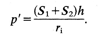
The relationship between wall-stress and ventricular cavity pressure can be visualized under static conditions by considering the forces acting on a small part of the ventricular wall. The situation is represented in Fig. 11.15.
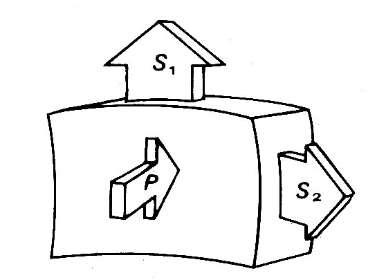
Fig. 11.15. Diagrammatic representation of the static force balance on a small part of the ventricular wall. P = ventricular pressure force, S1 and S2 = normal stress forces in wall.
The wall is loaded from inside by the ventricular pressure P. This is balanced by opposing forces within the wall, the most important components of which are stresses acting parallel to the wall surface (S1 and S2).* [* See also Chapter 7, where a similar force balance is described for blood vessels.] Because they act normally to the applied pressure force P they are called normal stresses; there may also be forces acting parallel to the cut surfaces, which will be tangential stresses.
The relationship between cavity-pressure and the wall-stresses is not simple for a number of reasons. These include the geometry, but are not exclusively related to it, and a consideration of the simplest possible shape - the sphere - will illustrate this.
If we wish to use simple elastic theory, we must first define the wall-stresses in a way which takes account of possible gradients of stress from the inner to the outer surface of the wall. As in Chapter 7, therefore, we must define stresses as the average values through the wall, since the gradients of stress which must exist are unknown. Thus the normal stresses (S1 and S2 in Fig. 11.15) are average values for the whole thickness of the wall. Next, we must assume that the wall is homogeneous and isotropic. Then, for the spherical shape, S1 = S2.
Now we can apply the law of Laplace, as in Chapter 7 (Equation 7.6) but bearing in mind that we are dealing with two mutually perpendicular normal stresses rather than the single hoop stress which describes circumferential tension in a tube. Thus Equation (7.6) becomes
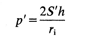
where p' is the pressure difference across the wall, ri is internal radius, and h is wall thickness; S' is equal to S1 and S2. If the material of the wall is not homogeneous and isotropic, a spherical shape is still possible, but S1 will not equal S2; then we shall have:
If we depart from a spherical shape, the simplest body of revolution to consider is an ellipsoid of revolution (for example, a rugby football). The situation here is potentially much more complicated, because tangential forces have to be taken into account. However, if we choose an element aligned along the principal axes of the ellipsoid, as in Fig. 11.16,
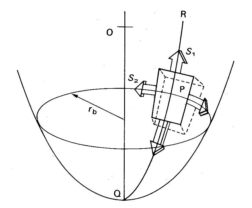
Fig. 11.16. Wall stress in ellipsoidal model of left ventricle. See text for details.
the tangential forces drop out and we can again write an equation linking transmural pressure with wall-tension:
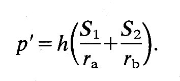
S1 and S2 are the normal stresses, as before; but ra and rb are not simple radii. The former is the radius of curvature of the surface in the longitudinal plane at the point P. This radius of curvature will obviously change continuously if P moves longitudinally over the ellipsoid, being tiny at the tips and largest on the equator. The second radius rb is the perpendicular distance from the axis of the ellipsoid to the point P. It will also vary continuously as the chosen point moves longitudinally and will only be a true radius (the minor axis radius) when P is on the equator of the ellipsoid. When it is at the tip it will be equal to zero.
11.4.1 Left ventricular shape and wall-stresses. It will be apparent from all this that when the body departs from a spherical shape even the simplest elastic theory will predict complicated relationships between transmural pressure and wall-stresses. It is thus hardly surprising that in many studies of the left ventricle a spherical shape has been assumed. In the very earliest, thin-walled spherical models were adopted, but these are hopelessly inadequate, not least because even in diastole the left ventricular wall-thickness is 20-30 per cent of the external radius, and during systole it is 10-12 per cent thicker than during diastole. The next model to be considered was the thick-walled sphere. This is reasonable in terms of the length-changes which the muscle-fibres must undergo; if the contained volume of such a sphere were halved during systole (which is approximately true in the ventricle) then fibres of the innermost wall layer would have to shorten by about 20 per cent. This is compatible with what we know of the normal sarcomere length range. Of course, the wall will thicken when the ventricle contracts, since muscle is incompressible, and the radius of the outer wall will be reduced by less than 20 per cent. Thus the shortening which individual fibres undergo will vary continuously through the wall from a maximum at the inside. This is of course a property of all thick-walled structures, as is the stress distribution referred to earlier.
However, although the spherical model is simple, and the length-changes reasonable, it is an unrealistic shape to adopt. It has been demonstrated by a number of methods that the shape of the left ventricle is complicated, both in man and in experimental animals. The clearest demonstrations of this come from cine films taken during continuous X-ray screening of the heart when radio-opaque water-soluble media are injected through a catheter whose tip lies in the cavity of the ventricle. (This technique, which is called cine-angiography, is widely used both clinically and in the research laboratory to examine the structure and function of the heart and blood vessels.) The left ventricle is revealed in this way (Fig. 11.17)
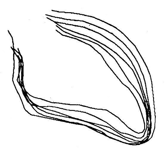
Fig. 11.17. Outlines of human left ventricular cavity (traced from cine-angiograms) at equally spaced intervals between end-diastole and end-systole. The outflow tract to the aorta is at the top left and the apex of the ventricle at the bottom right. (From Gibson and Brown (1976), personal communication.)
to be shaped rather like a blunted arrowhead, the apex forming the point of the arrow and the two valves forming its base. The inner wall of the ventricle is irregularly corrugated by longitudinal columns of muscle of varying thickness, and the papillary muscles project into the cavity to complicate its shape still further. In the transverse plane, the ventricle has usually been found to be roughly circular, and at normal diastolic volumes it has a diameter which is about half the length of the long axis.
When the ventricle contracts, the long axis first shortens slightly and the transverse diameter increases correspondingly. This happens before ejection begins, and probably results from contraction of the longitudinally orientated muscle fibres in the innermost part of the heart wall; electrical studies have shown that depolarization of the ventricular muscle starts at the inner wall. When ejection commences, the main change is a shortening of the transverse axes, which reduce by about a third; but this is asymmetric and there is more movement in the antero-posterior semi-axis than in the other; the long axis only shortens slightly. By the end of systole, the ratio of long to short axes is about 2.5:1. The changes which take place during contraction are summarized in Fig. 11.18,
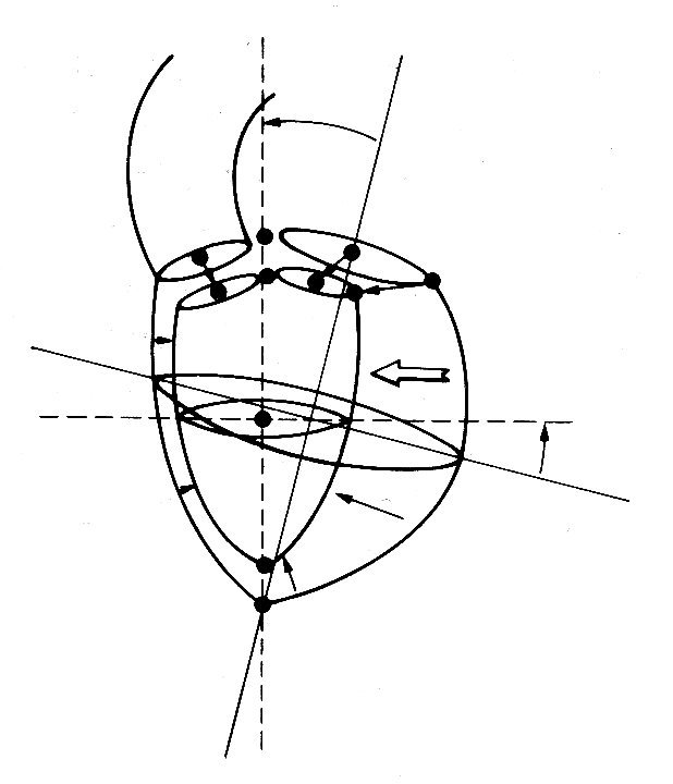
Fig. 11.18. Diagrammatic summary of the external dimensional changes and movement of the left ventricle of the dog from the end of diastole to the end of systole. The arrows indicate the distance and direction of wall movement. (After Hinds et at. (1969). 'Instantaneous changes in the left ventricular lengths occurring in dogs during the cardiac cycle'. Fedn Proc. Fedn Am. Socs Biol. 28, 1351.)
which is reconstructed from a study in which X-rays were used to follow the movement of radio-opaque markers attached to various points on the ventricular walls.
It is clear from these descriptions that the sphere is an unrealistic shape to adopt, since not only does the ventricle have long and short axes, but also the former hardly varies during the cardiac cycle. Recently, and much more successfully, ellipsoidal models have been used in which the long axis is assumed to be constant in length, volume changes being brought about by shortening of the minor axes; this fits quite well with the observations described above in the real ventricle. The amounts of muscle-fibre shortening required in this model are again compatible with known sarcomere properties—halving the contained volume of an ellipsoid of revolution, without shortening of the major axis, means that the minor axis, and therefore the circumferential fibres, must shorten by a maximum of 29 per cent at the inner wall. Finally, this model predicts wall-stresses which are closer to values obtained by direct measurement with force transducers than do spherical models.
However, one limitation still applies; these studies must assume uniform properties through the wall of the model. This ignores both the architecture of the ventricular wall (see Fig. 11.4) and the possibility of different degrees of active tension in differently stretched muscle-fibres. In a recent and comprehensive study,* these factors also have been incorporated. [*Streeter, D. D. Jnr, Vaishnav, R. N., Patel, D. J., Spotnitz, H. M., Ross, J. Jnr, and Sonnenblick, E. H. (1970). 'Stress distribution in the canine left ventricle during diastole and systole', Biophysical Journal, 10, 345-63.]
In this study, it is once more assumed that the ventricle is ellipsoidal, and also that the muscle-fibres can only bear tension axially. It is easy to see that the curvature of the muscle fibres in the wall of the left ventricle will be extremely complex, since they have a continuously varying direction through the curved wall (see Fig. 11.4). Therefore fibre-orientation and the principal radii of curvature of the ventricular walls were measured in post-mortem dog hearts, and the data used to calculate fibre-curvatures through the wall. These results were then used to calculate the distribution of normal and radial stresses through the wall, treating the wall as a tethered set of nested ellipsoidal shells, each shell having a single fibre-orientation which corresponds to the experimentally determined orientation at that level in the wall. Fibre curvature is found to be greatest in the mid-wall region at the end of systole, and towards the endocardium during diastole. The pressure or radial stress distribution is slightly non-linear through the wall if constant fibre-stress is assumed, the pressure decreasing most rapidly in the inner layers of the wall. If constant fibre-stress is not assumed in systole (and we know - e.g. from Fig. 11.9 - that active tension is length-dependent, and also that systolic sarcomere length varies through the ventricular wall) then pressure distribution across the wall is predicted to be approximately linear. The calculated distributions of normal stresses in the two principal axes during diastole and systole are shown in Fig. 11.19;
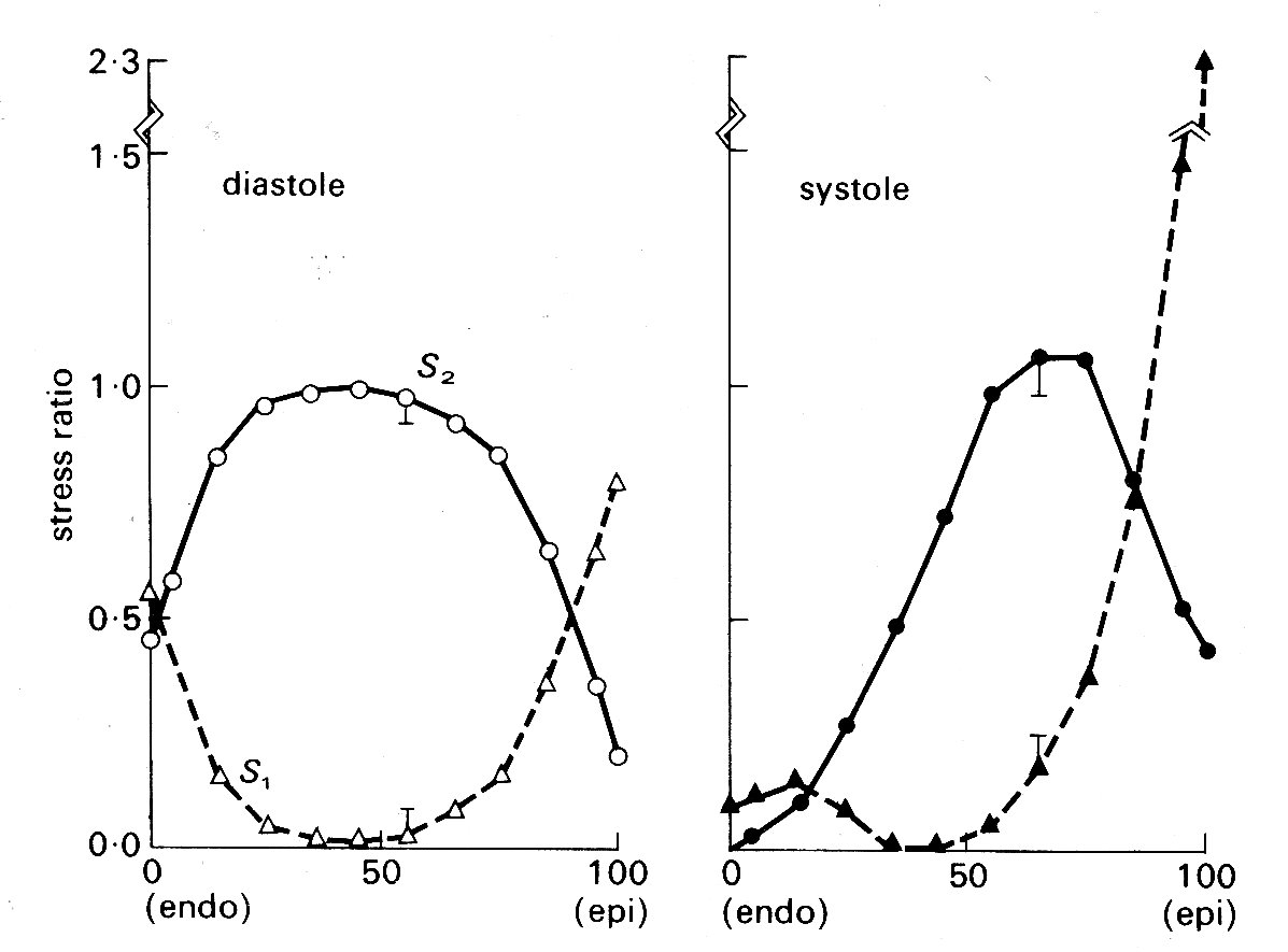
Fig. 11.19. Stress ratios in the left ventricular wall at the end of diastole and the end of systole. Abscissae: position through the ventricular wall from endocardial (0) to epicardial (100) surface. Ordinates: stresses, expressed as fractions of the average stress for the whole wall thickness. S1 - longitudinal stress S2 - circumferential stress (see Fig. 11.16) (After Streeter, Vaishnav, Patel, Spotnitz, Ross Jr, and Sonnenblick (1970). 'Stress distribution in the canine left ventricle during diastole and systole'. Biophys. J. 10, 357.)
again the fibre stress is assumed to vary through the wall during systole, but to be constant in diastole. The very great importance of allowing for fibre-orientation in studies of this kind is apparent; in models which assume homogeneous wall-properties, both longitudinal (S1) and circumferential (S2) stresses are found to be highest at the endocardial surface.
As part of the study, predicted values of circumferential forces were compared with values obtained directly in vivo with force transducers; good correspondence was obtained and even with the assumption of an ellipsoidal shape, such models of the left ventricle are clearly realistic and useful, though we may expect to see them modified as more detailed recent information about fibre geometry in the left ventricle,* and more accurate measurements of sarcomere length-tension relationships, are incorporated. [* Streeter, D. D. Jnr, Powers, W. E., Ross, Alison M., and Torrent-Guasp, F. (1976). "Three-dimensional fibre-orientation in the mammalian left ventricular wall', in Cardiovascular System Dynamics, eds. J. Baan, A. Nordergraaf, and J. Raines, M.I.T. Press, Cambridge, Mass.]
It should perhaps be emphasized that interest in a good model for the description of left ventricular wall-stress distribution has a very important practical basis, since the blood supply which nourishes the heart muscle is carried in the coronary vessels which run within the wall and are therefore subjected to the local wall-forces. Pressure and flow within the wall are, for technical reasons, difficult both to measure and to interpret, and our knowledge of the distribution of coronary blood flow remains very incomplete. The major part of flow from the aorta into the coronary arterial bed certainly takes place during diastole (Fig. 11.20),
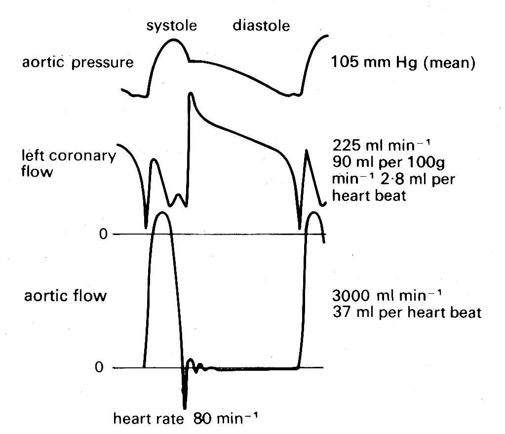
Fig. 11.20. Recordings of pressure and flow in the aorta, and flow in the left coronary artery. Measurements made in a conscious dog, fourteen days after surgical implantation of flowmeters. Note that flow in the coronary artery is predominantly diastolic. (From Gregg and Fisher (1962). Handbook of physiology. Section 2, p. 1534.)
as might be expected since intraventricular pressure and therefore intramural pressure are low compared with aortic pressure; and this diastolic flow is evenly distributed through the heart muscle. In systole the situation is more complicated, since the pressure within the inner layers of the ventricular wall must be close to that within the cavity, and it is difficult to see how blood flow into these layers can be maintained, since some frictional (viscous) pressure drop must occur in the coronary vessels. In fact a number of workers have made pressure measurements within this inner (subendocardial) wall region and have found that during systole intramural pressures may actually exceed intraventricular pressure. This is quite possible if fibre-orientation is not uniform. It could arise, for example, if a group of fibres developed a curvature opposite to that of the main body of the ventricular wall, either naturally or as an experimental artifact, and a similar result can be obtained in mathematical models by allowing this condition.
11.4.2 Right ventricular shape. The way in which the right ventricle contracts is much less clear because very little study has been devoted to it; but the pumping action is different from that of the left. One wall of the right ventricle—the septum—is functionally part of the left ventricular wall. The other, free wall is much thinner, and has a larger area, so that the cavity of the right ventricle is wrapped around one side of the left ventricle like a pocket, opening at the top into the pulmonary artery and right atrium. The area of the walls is thus large in comparison with the volume contained between them, and a relatively slight movement of the walls towards each other will displace a large volume.
This bellows action certainly takes part in right ventricular ejection, but may be augmented by two other mechanisms. The first has been convincingly demonstrated by X-ray studies of the motion of the free wall of the right ventricle. During systole, the free wall moves downwards, that is to say tangentially to the blood contained in the chamber. During diastole, it moves upwards again. The scale of this movement increases with distance'from the apex of the ventricle; thus the free wall behaves like an elastic membrane, anchored at the apex and stretched longitudinally during diastole; when it contracts, it moves down over the contained blood like a sleeve, so that the blood comes to lie in the outflow tract beyond the pulmonary valve. The principle of this type of pump, which can operate without a change in chamber volume, is illustrated in Fig. 11.21.
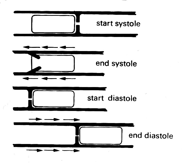
Fig. 11.21. The principle of a check-valve pump, which operates without volume change of the pumping chamber. The pumping action occurs by a change in position of the chamber and appropriate valve action. Emptying of the right ventricular outflow tract in dogs may be accomplished in part by such a mechanism. (From Carlsson (1969). 'Experimental studies of ventricular mechanics in dogs using the tantalum-labeled heart'. Fedn Proc. Fedn. Am. Socs. Biol. 28, 1324 )
The other mechanism which may contribute to right ventricular ejection is the contraction of the left ventricle itself, which will exert traction on the free wall of the right ventricle as the radius of curvature of the left ventricular wall decreases. How much importance this has is conjectural, since it has not been demonstrated radiologically; this is not surprising, since the relative motion which it would cause in any one plane would be small, and would occur very rapidly at a time when the whole heart is moving. There is, however, good evidence from both animal experiments and clinical observations that right ventricular function can be surprisingly well preserved in the presence of severe damage to the muscle-fibres of the right ventricular wall.
11.4.3 The mechanics of the entire ventricle. If we know the shape of the ventricle, we can begin to calculate for it the quantities which define the behaviour of isolated heart muscle. This way of examining cardiac performance treats the ventricle as a specialized muscle, whose geometry and mechanical properties will be the important determinants of contraction. Since this follows logically on earlier sections, we will deal with it first; but there is a second approach which we shall consider subsequently (although historically its takes precedence). This treats the ventricle as a pump, ignoring detailed mechanics and examining empirically the relationship between input and output and the factors which affect it.
The central feature of this latter approach is an experimentally derived input-output relationship known as Starling's law of the heart, which still remains an extremely valuable basis for understanding many aspects of cardiac function. It is, to a considerable extent, complementary to the muscle mechanics approach, and in recent years the tendency has been to try to unify these two approaches and describe ventricular pumping in terms of the instantaneous relationship between load and muscle-properties. As we shall see, the difficulties are great and this sort of synthesis of ventricular function is so far very incomplete.
Performance as a muscle. There are strong grounds, as we have seen, for thinking that the shape and movement of the left ventricle are geometrically much simpler than those of the right; and much of what follows relates to the left ventricle (though Starling's law certainly applies to the right ventricle also). If we accept that the shape of the left ventricle can be realistically described by an ellipsoidal figure, whose minor axes shorten during systole but whose long axis is constant, we can begin to calculate tension and velocity of shortening of muscle-elements in the wall. Average hoop tension in the plane of the minor axes can be derived from ventricular pressure if wall-curvature and thickness are known. The velocity of shortening of a circumferential wall-element in this plane can be calculated from the rate of ejection of blood into the aorta if the shape of the ellipsoid is known. Finally, the instantaneous length of the minor circumference can be calculated if the ejection-rate and the initial volume of the ventricle (end-diastolic volume) are known.
Experimentally, all this is an extremely tall order; in fact some of the required values can only be obtained indirectly. For example, end-diastolic volume cannot at present be measured accurately in the intact heart; it must be calculated from length measurements made with one or other of a variety of techniques such as X-rays, ultrasonics, or strain-gauges attached around the ventricle (or, with further assumptions, from the post-mortem heart). The situation is further complicated by the fact that the heart contracts neither isometrically nor isotonically: we must assume that shape changes are unimportant in order to treat the isovolumic phase as isometric, and that the afterload is constant throughout ejection if the ejection phase is to be considered isotonic. The former assumption is probably not too bad; the latter is undoubtedly crude, most obviously because aortic pressure is not constant throughout systole - see Fig. 11.5. More general assumptions which apply are that the ionic and chemical environment of the heart is held constant during the experiment, that the active state in each muscle-fibre begins instantly and remains constant throughout systole, and that all muscle fibres are activated synchronously.
In view of these problems, it is not surprising that there have been very few attempts to examine this problem in the normally beating intact heart. More often a special condition has been imposed (end-diastolic volume or aortic pressure held constant, for example, or the contraction rendered isometric by preventing the ventricle from ejecting) so that a particular facet of contractile behaviour, or a particular assumption about it, can be tested. Thus our knowledge of the intact ventricle, just as that of isolated heart muscle, is pieced together from many different kinds of experiment and is largely qualitative; the research literature is, predictably, just as voluminous and complicated as that which deals with the properties of isolated muscle-fibres.
It is difficult for several reasons to decide whether a hyperbolic relationship links muscle force and velocity of contraction. First, calculations of muscle-tension become extremely complicated if they are to take into account the complicated geometry and orientation of muscle-fibres in the heart wall, as we have seen above. In experimental studies, some average tension is usually calculated to represent muscle force. Secondly, it will be remembered that the force-velocity relation for muscle strictly applies only to the contractile element in muscle. Where tension can be held constant in a contraction, so that the series elastic component can be assumed to be at constant length, then the relationship will hold for the entire muscle; this condition often applies in isolated muscle experiments, and has led to the loose assumption that the hyperbolic relation applies to the whole muscle. In the intact heart, tension changes rapidly during contraction, and there will be times when the series element is lengthening while the contractile element shortens. Allowance for this must be made in calculating contractile element velocity, and to do so involves a whole new series of assumptions, including the use of elastic moduli derived from isolated muscle experiments to describe the series elastic element properties. A further complication in calculating shortening velocity also occurs. Because of the continuous nature of the muscle, shortening velocity has to be thought of as the rate at which a unit length of a given circumference is diminishing. The circumference chosen will be that for which tension is to be calculated; but since the ventricular wall is thick, the shortening per unit length of fibres at different radial positions will vary. This can be overcome by visualizing the wall as a series of infinitely thin shells, all changing volume at an identical rate; a spatial average for the shortening velocity can then be derived. The final limitation of this approach is that the performance of the intact heart can only be examined over a relatively small range of force and velocity.
Despite all these difficulties, it has emerged quite clearly that factors which are important to the performance of isolated cardiac muscle are also very relevant in the intact heart. This can be seen in Fig. 11.22,
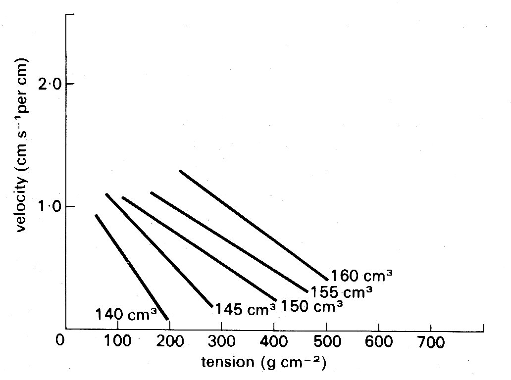
Fig. 11.22. Tension-velocity relationships for the intact ventricle calculated from experimental data for a series of ventricular volumes. Shortening velocity relates to the muscle contractile element, and is expressed per centimetre of circumferential length. (After Fry (1962). Fedn. Proc. Fedn. Am. Socs. Biol. 21, 991.)
in which the velocity of shortening of the contractile element in the intact heart wall is plotted against the instantaneous tension. In this experiment, the volumes and wall-thicknesses were calculated from measurements of surface segment-lengths in known planes, assuming an ellipsoidal shape for the ventricle; shortening velocity was calculated from measurements of the rate of ejection of blood into the aorta, and tension from measurements of left ventricular cavity pressure. Each line is derived from the values obtained at a single instantaneous ventricular volume. The scatter in such experiments is marked (not surprisingly, considering the experimental complexities, let alone the assumptions necessary for the calculations); nonetheless, two conclusions emerge clearly. First, there is an inverse relationship between velocity and tension at each ventricular volume, and secondly, the lines move upwards and to the right with increases in ventricular volume. If we accept the latter as being analogous to increases in fibre-length, the similarity between the behaviour of the intact heart in this figure, and the isolated muscle preparation in Fig. 11.14, is striking.
Since results like this have been obtained in a number of different kinds of experiment, we can be confident that tension, initial fibre-length, and the velocity of shortening of the contractile element are important determinants of function in the intact heart. What remains a problem is that in many experimental situations, and particularly in the clinical situation, these variables will not be known, or calculable, in precise form. It has therefore been necessary to use more easily measured parameters which reflect changes in these fundamental properties. Some of these have already been mentioned; but they assume such experimental importance that it is worth considering them in a little more detail.
We have already seen that ventricular volume is usually used to represent muscle-fibre length when we consider the intact heart; and that the relationship between these two is a statistical one - in the sense that volume is representative of some average fibre-length - because of the complicated geometry of the ventricle. It has also been mentioned that ventricular volume is difficult to measure in the living heart. However, this is not true of pressure, and it is common practice to use the diastolic ventricular pressure as a yardstick of ventricular volume and therefore of resting muscle-length; for this reason the end-diastolic pressure is frequently referred to in the literature as the 'preload', by analogy with the resting tension in isolated muscle. Clinically, resort is frequently made to a further approximation. It is assumed that at the end of diastole the atrioventricular valve is still open, but little or no flow is occurring, so that pressure in the atrium will be equal to that in the ventricle. This is particularly useful for the right side of the heart, where the pressure in the veins can be crudely assessed visually by leaning the subject back and using the veins in the neck as a manometer ('jugular venous pressure') or measured accurately by passing a fine catheter from a vein in the arm or neck into the large veins within the chest or the right atrium to measure 'central venous pressure' or 'filling pressure'.
It should be obvious that the use of end-diastolic pressure to define the initial length of muscle in the ventricular wall is a purely qualitative method. For one thing, it assumes that the relationship between ventricular pressure and volume is independent of time - i.e. that it cannot alter in disease states, and that there is no 'creep' in the elastic properties of the ventricular wall. This latter assumption does not seem to have been critically tested; it may not be important in short-term experiments, and particularly those involving changes in filling from beat to beat, but creep is certainly observed in isolated heart-muscle at rest, and this may be relevant when the heart is distended in diastole for long periods. A further point which is sometimes forgotten is that it is the pressure difference across the ventricular wall ('transmural pressure') which dictates how stretched it is, and if the chest is intact the pressure outside the ventricle varies with breathing. During inspiration, for example, the pressure within the chest becomes sub-atmospheric, and so may that within the ventricle if its transmural pressure is low. This is not too extreme an example; the end-diastolic pressure range in the normal left ventricle is of the same order as the swings in intrathoracic pressure which occur even during quiet breathing.
Nowadays, measurement of end-diastolic pressure in man with catheters is technically straightforward. Large ventricular volumes are a common feature of human heart disease, particularly heart failure, and therefore all the above considerations are of practical importance. An important recent advance has been the development of ultrasonic devices that function like depth-sounders on ships and can be applied to the chest wall to examine left ventricular dimensions ('echocardiography'). These can follow ventricular wall movement (and hence the velocity of muscle shortening) throughout the cardiac cycle. Thus they offer a non-invasive means of assessing chamber size, as well as, in conjunction with catheter pressure measurements, a potential means of examining pressure-volume relationships directly in many experimental and clinical situations.
In summary, the end-diastolic pressure can be extremely useful in describing the initial conditions from which the ventricle contracts in any experiment, although we cannot rely on its absolute level being uniquely related to resting muscle-fibre length. In practice, it has been invaluable in studies of the intact heart, particularly as a simple means of monitoring the resting length of the muscle in the heart wall.
Thus the need for volume-measurement, as an index of muscle-fibre length, can be at least partially side-stepped in diastole by the use of end-diastolic pressure. In systole, when ventricular volume changes with ejection, the problem crops up again. Here, it is experimentally more manageable, since the rate of ejection of blood from the ventricle can be measured in a variety of ways in experimental animals, for example by the use of flow meters attached to the aorta or pulmonary artery (the method used to obtain the flow records in Fig. 11.6); the measured flow-rate is obviously related to the shortening velocity of muscle-fibres. However, there are still complications. For geometrical reasons the relationship will be non-linear; for example, if we use the ellipsoidal model with a fixed major axis described earlier, then the minor axis, and therefore segments of the circumference, shorten proportionally to the square root of the volume change, and the absolute shortening is dependent upon the initial length of the axis. Thus once again there are geometrical problems in relating the behaviour of the whole ventricle quantitatively to that of the muscle-fibres.* [*If we wish to be really rigorous in examining the applicability of muscle-fibre models to the performance of the intact ventricle, then we must know the velocity of shortening of the contractile element of the muscle, rather than that of the whole fibre; to do this we must either assume that tension is constant through systole (so that the series elastic element is at constant length) or use information about the series element derived from isolated muscle experiments to adjust the velocity of shortening of the whole fibre; even this approach, which was used in deriving Fig. 11.22, is obviously not wholly satisfactory, because it assumes that quantitative results obtained in a very artificial experimental situation are applicable generally in the normal heart.]
In man, instantaneous aortic flow cannot be measured except in very special circumstances, and the only solution is to measure cardiac output, using a standard method such as indicator-dilution. This will give a value for volume flow-rate which is averaged with respect to time; it can be divided by heart-rate to give stroke-volume but it cannot be used to describe instantaneous events during systole.
The load against which this volume of blood is ejected from the ventricle is the third parameter of interest, and is in many ways the most difficult to treat realistically. When the ventricular pressure has risen sufficiently in early systole to just exceed aortic pressure, the aortic valve opens and ejection (muscle-shortening) begins. It is easy to see the aortic pressure (which only differs very slightly from ventricular pressure in normal systole -see Fig. 11.5) during this phase as analogous to the 'afterload' against which the isolated muscle shortens in Fig. 11.12, just as end-diastolic pressure is analogous to the 'preload' which sets the initial length and tension of the muscle.
However, as we saw earlier, we can only describe the load on the ventricular muscle in a way which is analogous to the load applied in isolated muscle-fibre experiments if we replace cavity pressure by wall-stress. These are related through the geometry, volume and wall-thickness of the ventricle, and the latter two, as well as the pressure, are changing throughout ejection. Ventricular volume goes down fairly steadily throughout systole; but ventricular pressure rises and then falls (Fig. 11.5). Thus if we assume elastic properties for the ventricle, and look at circumferential stress, it may be fairly constant in early systole, but later on the decreasing radius of curvature and increasing wall-thickness will tend to reduce it; thus tension will fall faster than the pressure (see Equation (7.6)). In other words, the pressure-volume relationship for the contracting ventricle will have a different shape from the length-tension relationships of isolated muscle-fibres, and the use of systolic pressure as a way of describing the load at muscle-fibre level will at best be very crude. Again, we are up against a geometric separation between the quantities which can be measured and those which determine the performance of the muscle-fibres.
In summary, the properties which determine the behaviour of isolated samples of ventricular muscle also operate to determine the behaviour of the intact heart muscle; but in the practical study of the heart the properties of the muscle are separated from the properties of the intact chamber by a series of uncertainties - largely geometric - and descriptions of ventricular function cannot usually be presented in terms of the fundamental muscle properties which have been described in this chapter.
Performance as a pump. There is, however, an alternative approach, which is to treat the heart as a pump rather than a muscle, describing its performance empirically. This approach is much older; its foundations were laid in the latter part of the nineteenth century by the German physiologist Frank, and elaborated some years later in England by E. H. Starling. Thus it has exclusively experimental origins, and its main ideas predate our knowledge of muscle mechanics.
The main theme of these early experiments was to examine the relationship between the input and output of blood to the heart. Frank worked on the frog's heart, using rather crude methods; but Starling achieved an enormous experimental success in developing the heart-lung preparation, in which the working heart and lungs of an anaesthetized animal could be disconnected from the circulation to the rest of the body. Thus the blood ejected from the left ventricle into the aorta was collected in a reservoir and returned to the heart via the right atrium. With this preparation, it was possible to control independently both the filling pressure of the atrium and ventricle and the aortic pressure. Starling found that as the inflow of blood to the atrium was increased, so the atrial pressure gradually rose, and so did the cardiac output (Fig. 11.23).
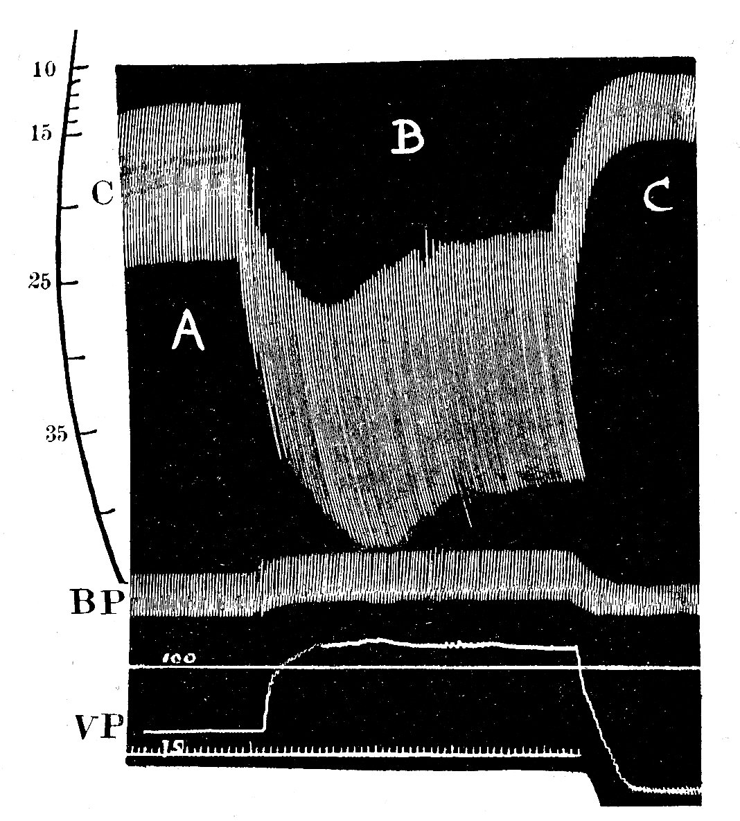
Fig. 11.23. Reproduction of one of Starling's original figures, showing the effect of an increase in venous filling pressure (VP) on diastolic and systolic heart volume in the heart-lung preparation The records were made with a smoked drum recorder. The top trace (C) is a continuous record of ventncular volume (made by a displacement technique, the ventricles being contained within a rigid chamber); calibration in millilitres. Middle trace (BP) is arterial pressure in mm He with calibrations below at 100 and 75 mm Hg. Lower trace (VP) venous pressure (uncalibrated) Time marker in seconds.
A. Control period. Venous pressure 95 mm H20. Ventncular output 520 ml min-1
B. Step increase in venous pressure to 145 mmH20. Note corresponding increase in both ventncular diastolic volume and stroke volume. Ventncular output 840 ml min-1
C. Step decrease in venous pressure to 55 mm H20. Both diastolic and stroke volumes fall below control. Ventncular output 200 ml min-1 .
(From Patterson, Piper, and Starling (1914). 'The regulation of the heart-beat'. J. Physiol. 48, 465.)
The relationship was not linear; successively smaller increments of output followed each equal increment in venous pressure, until in some cases the output actually began to diminish. He went on to demonstrate that this effect occurred on each side of the heart, so that when the right side of the heart increased its output in response to an increase in filling, this extra output was applied to the left side of the heart where the same effect followed. In a further series of experiments, in which changes in ventricular volume were also measured, he showed that when the heart had to do more work because the aortic pressure was raised, the stroke volume at first fell, so that the ventricle was enlarged; thereafter the stroke-volume was restored to its previous value.
From our present knowledge of the mechanics of cardiac muscle (which dates fom the late 1950s) we can see that Starling was demonstrating the behaviour of cardiac muscle when it shortens from different initial lengths, and we have at least some clues, from the ultrastructure of the sarcomere, about how this may work. It is a measure of the insight which Starling brought to bear on the behaviour of the heart that he concluded (in 1914): 'The law of the heart is therefore ... that the mechanical energy set free on passage from the resting to the contracted state depends on the area of "chemically active surfaces", i.e. on the length of the muscle-fibres.'
Thus Starling's law of the heart (or the Frank-Starling mechanism, as it is alternatively known) described the important relationship between initial filling of the heart (i.e. muscle-length) and the volume of blood ejected. The relationship was expressed in very loose mechanical terms - words like 'energy' and 'work' being poorly defined - but it clearly established the way in which the output of the two 'series' pumps which make up the mammalian heart are matched, and how they can respond to changes in filling pressure (preload) and arterial pressure (afterload) through the same basic mechanism. In brief, Starling showed experimentally that both sides of the intact heart are intrinsically capable, over a wide range of conditions, of ejecting whatever volume of blood is returned to them.
Starling himself was well aware of the limitations of this description of cardiac function. The obvious one is that it is not quantitative; even in a single heart, the absolute level of the relationship between filling pressure and cardiac output may vary. For example, in the second experiment mentioned above, the increase in ventricular volume which follows a step-up in aortic pressure may be followed, after a few beats, by gradual reduction of ventricular end-diastolic volume (i.e. filling pressure) back to its previous level, without any drop in cardiac output.
Starling thought this was due to an increase in coronary blood flow, and thus 'improved nourishment of the muscle'; in fact, the effect occurs even if coronary flow is held constant and its cause is probably related more to improved distribution of blood in the myocardium, so that the inner layers are better nourished. For our purposes, it serves merely to demonstrate that the relationships between filling pressure and output of the ventricle may be influenced by the load, and if we wish to express this graphically we need a series of curves showing the relationship under different loads - i.e. different mean arterial pressures. Again, this can be done using three axes to the graph, as in Fig. 11.24.
Fig. 11.24. Cardiac output in the dog heart-lung preparation, expressed in terms of venous filling pressure and aortic pressure. Note that over the physiological range of pressures cardiac output is sensitive to changes in filling pressure (preload) but not arterial pressure (afterload). From Herndon and Sagawa (1969) Am. J. Physiol. 217, 65.)
Since Starling's original experiments, it has been shown that the fall in output which may follow when an already high filling pressure is further increased (and which was regarded in clinical circles for some years as the basic mechanism of heart-failure, attributed to elongation of the muscle-fibres beyond some functional limit) is actually due to incompetence of the atrioventricular valve, which is overstretched by the great distension of the ventricle so that a portion of the ejected blood passes back into the atrium.
The experiments have also been repeated, in a wide range of conditions, using left ventricular end-diastolic pressure as the index of filling, and stroke work as the index of the 'forcefulness' of contraction (Fig. 11.25).
Fig. 11.25. Ventricular function curve. showing the relationship between left atrial mean pressure and left ventricular stroke work. (From Sarnoff (1955) Physiol. Rev. 35, 107.)
Stroke work is here defined as stroke volume times mean aortic pressure and thus has the correct dimensions of force x distance to describe external work; it was introduced as an alternative measure of ventricular function to Starling's simple stroke volume for two reasons. First, Starling presented many of his conclusions in terms of energy, so that work (which has the same dimensions) seemed an appropriate index to use. Secondly, work takes account, at least crudely, of the load against which ejection occurs, because it includes mean aortic pressure. In the heart-lung preparation where aortic pressure is controlled, and can be held constant, this is valid; but in studies of the intact circulation stroke work must be used with great prudence, since the aortic pressure is not related in any direct way to end-diastolic pressure. For example, stroke work does not remain constant as aortic pressure is varied; it goes from zero when the ventricle ejects with no opposing pressure, up to a maximum, and then down again to zero when pressure is high enough to prevent ejection completely. Since aortic pressure in the intact circulation reflects the properties of the peripheral circulation as well as the effects of ejection, stroke work may be a highly unreliable index of cardiac performance. There are also other reasons why stroke work is a very imperfect way to describe myocardial performance. For example, it takes no account of either external work in setting the blood in motion, or internal energy losses (e.g. due to friction) in the muscle.
When conditions are controlled appropriately, such studies demonstrate (as Starling implied, though never specifically stated) that the curve relating end-diastolic pressure and stroke work (usually known as the 'ventricular function curve') is not a single entity; rather a family of such curves exists for any particular heart, so that some other influence besides diastolic fibre-length must act to determine the performance of the ventricle.
This second determinant is usually described as the contractile state, or contractility, of the ventricle, and factors which affect it, as was briefly mentioned earlier, are known as inotropic factors; they may act either positively as shown in Fig. 11.26,
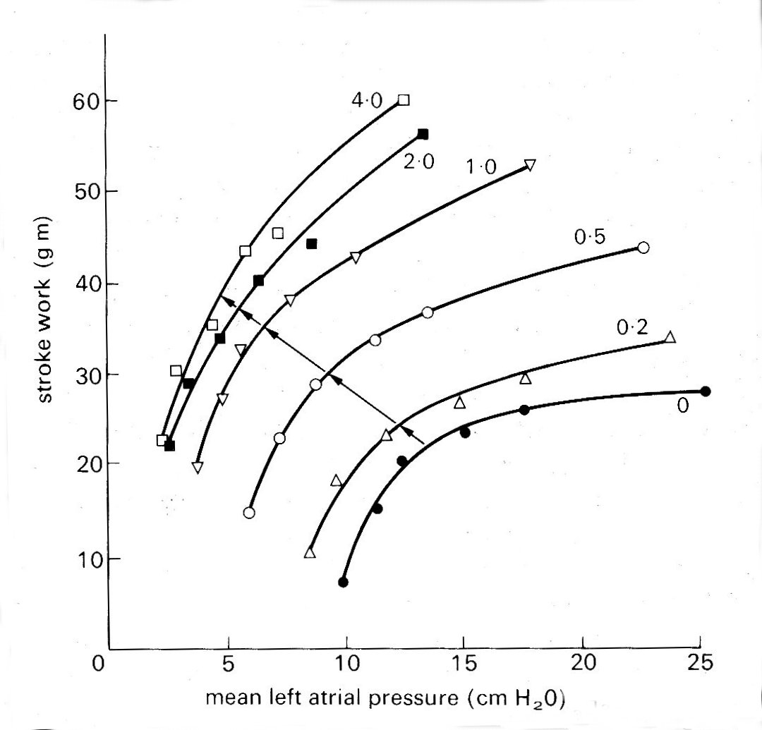
Fig. 11.26. The effect of sympathetic nerve stimulation, which has a strong positive inotropic effect, on ventricular function in the isolated heart-lung preparation. Each curve shows the relationship between mean left atrial pressure and left ventricular stroke work (the 'ventricular function curve ) at successively increasing frequencies of stimulation of the sympathetic nerves to the heart (stimulus frequency in shocks per second, marked on each curve) (From Sarnoff and Mitchell (1961). Am. J. Med. 30, 747.)
displacing the ventricular function curve so that stroke volume or stroke work at a given left ventricular end-diastolic pressure is augmented, or negatively. Such shifts of the curve are usually described as changes in contractility, and may be the end result of many different sorts of influence such as temperature, blood supply, oxygenation, and ionic and chemical environment. Among the chemical influences, the most important group of positive inotropic agents (which may well have a final common path in the energy release processes within the muscle-cell) are the catecholamines, naturally occurring or synthetic substances similar to the hormone adrenaline. One of these, isoprenaline, has a particularly powerful influence, and is widely used both in the laboratory and clinically for this reason. Stimulation of the sympathetic nerves which supply the heart has a similar effect on ventricular performance (probably acting via adrenaline released at the nerve-endings in the heart); a number of drugs, and increased concentrations of calcium and other ions in the circulating blood, all augment the contractility of the heart. Sympathetic nervous activity, and the release of adrenaline into the blood from the adrenal gland, are normal components of a range of responses (usually categorized as 'fight or flight') in animals, and of both physical and emotional stress in man. Their importance as a determinant of the behaviour of the normal heart, complementary to the Frank-Starling mechanism, has only comparatively recently been recognized. Starling's original findings, which related venous filling and cardiac output, were immediately accepted, but were only extended in this way after almost forty years. In fact the recognition of the effect which adrenaline or sympathetic nerve stimulation has on ventricular function, and the emergence of the concept of 'contractility', roughly coincided with the development of knowledge about the properties of isolated heart muscle.
The concept brought with it great difficulties. The first was one of definition. It is easy to see how, say, sympathetic nerve stimulation may 'set' the ventricular function curve at different levels, as in Fig. 11.26; but we cannot define the effect by saying that an increase in contractility causes an increase in stroke volume from a given end-diastolic pressure, because a fall in aortic pressure might do exactly the same thing (see Fig. 11.24) and its cause might have nothing to do with the heart. Thus the definition of contractility in this way first requires a description of the ventricular function curve, and this is obviously very cumbersome. Furthermore, it is extremely difficult experimentally to study contractility in terms of the ventricular function curve, because rigorous control of sympathetic nervous activity, end-diastolic pressure and aortic pressure is necessary before an effect on stroke volume or stroke work can be attributed to a change in contractility. Finally, quantitative comparison between cardiac performance in different experiments is very difficult.
For these reasons, and because of the growing realization that cardiac muscle performance could be described more fundamentally in terms similar to those which applied to skeletal muscle, attempts to describe the heart as a pump lost impetus, and the search began for some means of quantifying the contractility of heart muscle among the force-velocity-length properties we have described earlier in this chapter.
The ultimate objective was, of course, to find some index which could be applied to the intact heart, both experimentally and clinically. We have already seen the difficulties which surround the application of muscle mechanics to the intact ventricle, and it is not surprising that 'contractility' still remains an ill-defined quantity in the intact heart. In isolated muscle preparations, on the other hand, it can be defined: here the influence of length changes can be eliminated by doing experiments at constant length, and it can be shown that changes in the inotropic state of the muscle are reflected in alterations in the force-velocity curve, as shown in Fig. 11.27;
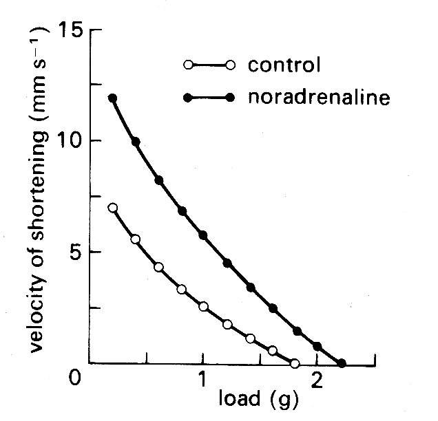
Fig. 11.27. Effect of a positive inotropic intervention (the addition of noradrenaline to the perfusing bath) on the force-velocity relationship of isolated heart muscle. Initial muscle length held constant throughout. (From Sonnenblick (1962). Am. J. Physiol. 202, 931.)
again, positive influences give an upward shift to the curve. Thus an inotropic influence was denned as one which displaced the force-velocity curve when acting on a muscle at constant length. This immediately suggested that one or other of the intercepts of the force-velocity curve might be used as an index of the contractile state of the muscle, because it might be possible to extrapolate to get either the force at zero velocity (isometric force, P0) or the velocity of contractile element shortening at zero load (Vmax).
There are insuperable difficulties in trying to use isometric force. We have already seen the difficulties and assumptions which arise in calculating wall-force from cavity-pressure; and for the present purpose it is also essential to be sure that length-changes in the muscle (i.e. changes in end-diastolic volume of the ventricle) do not occur between measurements. (The very powerful effect of initial muscle-length on isometric force can be seen in Fig. 11.14, where the points of interception on the load axis are isometric contractions.) Nor can we adopt the much simpler, though cruder, approach of equating maximum wall-force with maximum developed pressure in the ventricle, because the maximum pressure occurs after the valve has opened (see Fig. 11.4), when muscle-length is changing.
A much more optimistic view has always been taken of the practicability and validity of using Vmax as an index of contractility. This was chiefly because Vmax was thought to be independent of muscle-length - implying that all the curve's in Fig. 11.14 can be extrapolated back to the same velocity origin - whereas it can be demonstrated to depend strongly on inotropic state; i.e. the curves in Fig. 11.27 extrapolate back to different velocity origins. The assumption about the length-dependence of Vmax was discussed earlier (§11.3.4), and has been strongly criticized for the reasons given there; but the idea is still stimulating a great deal of work and controversy because of the practical value which an index of contractility would have and because the alternative approaches have proved fruitless.
Initially, the reasoning was that Vmax, calculated from the absolute level and rate of rise of ventricular pressure, with assumptions about the properties of the series elastic element, the synchronicity of contraction, and the geometry of the ventricle, would be an index of contractility which was independent of length changes in the ventricle (i.e. of the Frank-Starling mechanism). However, doubts have grown steadily in recent years about the constancy of Vmax with changes in initial fibre-length. This, together with the uncertainties and difficulties of the calculations involved, have directed interest towards simpler, more direct parameters which might change in the same direction as changes in contractility. The one which has received most attention is the rate of rise of ventricular pressure itself, which was one of the measurements necessary for the derivation of Vmax. The time-course of ventricular pressure and its rate of change (dp/dt) are illustrated in Fig. 11.28;
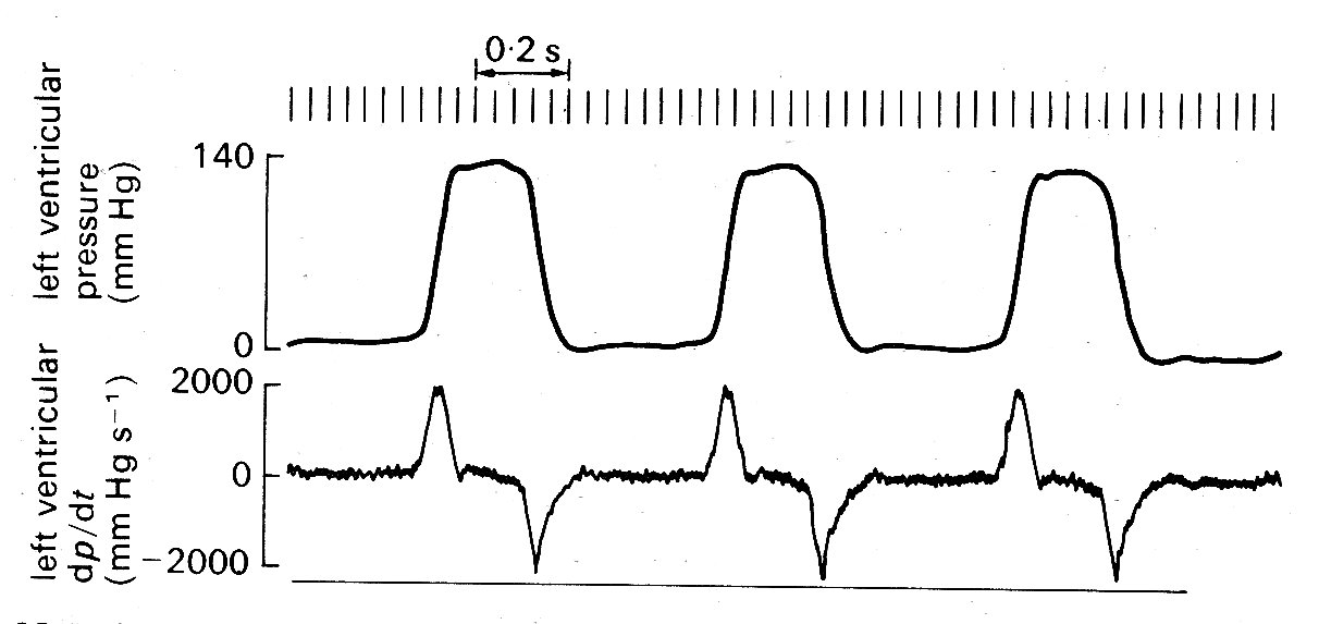
Fig. 11.28. Left ventricular pressure (upper trace) and its rate of change (lower trace). The pressure was recorded with a high-fidelity manometer mounted on a catheter tip and located within the ventricle; the rate of change was derived from this signal by electronic differentiation. (From Gabe (1972). Cardiovascular fluid dynamics, p. 14, Academic Press, New York.)
the rate of rise reaches a peak ('dp/dtmax') late during the isovolumic period, and since this might bear some relation to the maximum velocity of shortening of the muscle contractile elements, and certainly shows large changes in response to inotropic agents attention has been focused on it. Strictly speaking, dp/dt is not directly measured; it is derived by electronic differentiation from the ventricular pressure signal, which is directly measured. (The more traditonal method of drawing a tangent to the upslope of the pressure signal is highly unreliable because the duration of maximum slope is so brief - see Fig. 11.28) The pressure measurement must be free of distortion, which is difficult to achieve reliably with long fluid-filled catheter-systems; but with modern end-catheter manometers the measurement is practicable in man as well as in experimental animals.
Both the interpretation and the usefulness of measurements of dp/dfmax are currently being debated. The value should, for example, be affected by initial muscle-length since it is an expression of the rate of rise of wall-force, and we know that the latter is length-dependent. Furthermore, since dp/d^ax is reached late in the isovolumic period it might also be reduced if there was early opening of the aortic valve and the onset of shortening—e.g. if there was a low aortic pressure. In other words, it might be susceptible to afterload as well as preload. Most (but not all) investigations have suggested that dp/dt^ is affected by both these factors, and it is certainly far from being universally acceptable as an index of the contractile state of the ventricle; but it may prove to be of value in certain defined circumstances, for example, where aortic and left ventricular end-diastolic pressures are stable, or can be controlled. Meanwhile, the search for a generally acceptable and quantitative index of contractility continues, despite the views of the purists who have studied the problems of cardiac mechanics in detail and are convinced that no single such index can exist. The pragmatists, who are increasingly preoccupied by the need to assess cardiac performance in patients, are rightly (though optimistically) prepared to test empirically almost any promising parameter which can be measured. In the long run, what is probably needed is a biochemical measurement within the cell; the processes of energy-release in muscle, though not our concern here, are the subject of intensive and rewarding study and are steadily being clarified. In the meantime, however, the problem has to be tackled as a mechanical one.
11.4.4 Summary. The performance of the intact heart has been examined from two main points of view. The first, which takes historical precedence, looks at the heart as a pump and examines the relationship between input (usually measured in terms of venous or atrial pressure) and output (usually measured as stroke volume), without attempting to understand the underlying mechanisms.
In this view, blood entering each chamber of the heart stretches it and the contraction which follows ejects a volume of blood which is proportional to this stretch. This is known as the Frank-Starling mechanism (§11.4.3), and will account not only for control of heart output in response to venous return but for matching of output on the left and right sides of the heart. However, it is obviously an incomplete description of cardiac performance, because it takes no account of the load ('afterload') against which the heart must work in order to eject the stroke volume; to allow for this the relationship has been restated in terms of ventricular end-diastolic pressure and stroke work, which is defined as the product of stroke volume and mean aortic pressure, and is actually an incomplete measure of the external work done by ventricular muscle This relationship is known as the 'ventricular function curve'; it is not unique for any particular heart-chamber, since a third major influence, the contractile state of the muscle, also affects performance. Thus a family of ventricular function curves reflecting the influences of preload, afterload, and contractility are needed for a complete description of the heart's behaviour.
Conceptually, this approach has been tremendously useful - it is easy to visualize a curve relating input and output, whose position on a graph is adjusted upwards and downwards in response to variations in overall volume demand by the circulation. Experimentally, however, its usefulness is limited and in addition, since it treats all the parameters as time-averages, it cannot be applied at all to describe the course of events within a single beat. Thus it offers a clear, but very incomplete, description of events.
The second approach is to examine the heart in terms of muscle mechanics and to try to equate the properties described in isolated muscle-fibre experiments with the performance of the whole chamber. A series of extremely difficult and complicated transformations must be made to do this because of the complicated geometry of the ventricles and the fibre-orientation - in fact so far it has only been seriously attempted for the left ventricle. A considerable body of specialized evidence now exists to support the view that the properties found in isolated muscles do determine the behaviour of the intact chamber - but this is not yet a practicable approach to the assessment of cardiac performance at a clinical and experimental level because the necessary measurements are too difficult, and many of the assumptions too insecure. Unfortunately these limitations tend to be forgotten in the growing clinical demand for useful indices of cardiac performance, both for assessment of disease processes and tor the evaluation and guidance of surgical and medical treatment.
One final point needs to be stressed. All the functional descriptions in this chapter relate to the heart isolated from its circulation; we examine input and output pressure and flow exclusively from the point of view of the heart In the intact animal, the behaviour of the heart is continually modified, through the mechanisms we have discussed, by outside influence. Thus we may sometimes be in a position to predict the effect on the heart of a particular circulatory adjustment, but this is not true in reverse; the circulation is in a continuous state of reflex adaptation, both to the demands of the body tissues for blood and to 'feedback' mechanisms which respond rapidly to a range of stimuli like pressure and chemical factors in the blood. In other words, many phenomena occur in the circulatory bed of the body totally independently of the heart's performance.
11.5.1 Right heart. The factors governing flow into the right atrium are complicated, but the ultimate driving force is the arterial pressure. The pulsation which is seen in the aortic pressure has been largely smoothed out, and the mean level greatly reduced, during the passage of blood through the systemic microcirculation, but it is still high enough at the venous end of the capillary bed to generate a flow towards the heart. The smoothing which occurs means that this is basically a steady driving force; but a number of factors acting unsteadily superimpose oscillations upon the flow. Some of these, such as the 'muscle pump' (§14.5.2), are peripheral in origin, and cause oscillations of pressure which propagate primarily towards the heart. Others are secondary to pressure swings which occur within the chest due to breathing. Finally, there are pressure changes within the atrium itself, due to contraction of the heart, which add further pressure oscillations; these propagate back through the veins because of the absence of valves at the venous entrances to the heart (see Chapter 14).
Thus flow enters the right atrium in an unsteady stream and the pressure there, and in the adjacent veins within the thorax, fluctuates throughout the cardiac cycle even in a subject breathing quietly and at rest (Figs. 11.5, 11.29, and 14.20).
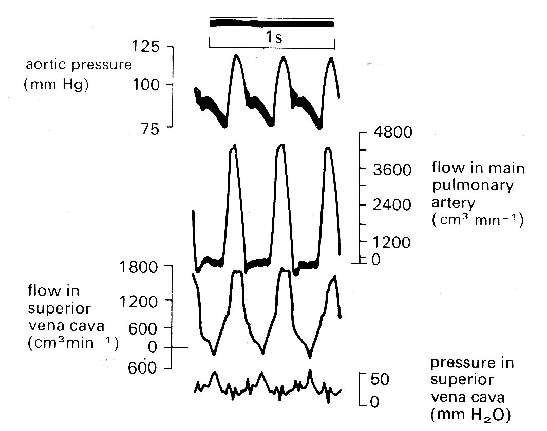
Fig. 11.29. Simultaneous records of aortic pressure, pulmonary artery flow, and superior vena cava flow and pressure. Note that in the SVC, maximum flow towards the heart (positive signals) occurs during ventricular systole, and maximum pressure (caused by right atrial contraction) coincides with a brief reversal of flow direction. (From Brecher (1956). Venous return. Grune and Stratton Inc., New York.)
The pressure waveform has two main components, the 'a' and 'v' waves. The former is due to atrial systole; the latter shows a slower rise, coinciding with ventricular systole and terminating with a rapid fall (the 'y' descent) when the tricuspid valve opens and flows into the ventricle takes place early in diastole. These fluctuations are visible in the jugular vein in the neck when a subject lies flat or nearly flat; and in disease, their form may give invaluable information about the functional state of the right heart. The mechanisms of venous flow into the thorax is dealt with in more detail in Chapter 14.
Flow within the right side of the heart has not been studied in detail. In view of structural similarities, it seems reasonable to assume that the valves behave like those on the left side, which will be dealt with in §11.5.2. On the other hand, the mechanics of right ventricular contraction are certainly different from those on the left, both in the way in which the volume change is achieved and in its time-course, which is slower (see Fig. 11.6). At the beginning of systole, pressure in the right ventricle rises more slowly than in the left; but the mean pressure in the pulmonary artery is so much lower than that in the aorta (10 mm Hg versus 100 mm Hg) that the pulmonary valve opens before the aortic valve, and ejection begins several milliseconds sooner. Both the acceleration and deceleration of blood in the pulmonary artery are much slower than in the aorta, and the peak flow-rate is also less. Thus the whole waveform is smoother and blunter (Fig. 11.6), ejection takes longer, and the valve closes later than the aortic valve. The second heart sound therefore has two components (Fig. 11.5).
The peak Reynolds number in the pulmonary artery, which is calculated from Equation (5.5), using peak systolic blood velocity, pulmonary artery diameter, and the kinematic viscosity of blood, is somewhat lower than in the aorta. Quoting exact figures is misleading, since there is a very wide range, probably even in normal animals at rest, and certainly as measured under different experimental conditions; but peak Reynolds numbers between 2000 and 4000 for the main pulmonary artery, and 2500-7000 for the aorta, are realistic. The question of the occurrence of turbulence in the circulation is considered later (§12.8.3.); the problem has not yet been experimentally studied in the pulmonary artery under normal conditions.
11.5.2 Left heart. Pressure and flow events in the pulmonary veins and left atrium differ in some respects from those in the systemic veins and right atrium, and are dealt with in Chapter 14. For our present purpose, which is to examine fluid mechanical events in the left atrium and ventricle, they can be considered as a reservoir, which fills up during ventricular systole and begins to empty into the ventricle at the beginning of diastole when the pressure gradient across the mitral valve becomes negative due to both rising atrial and falling ventricular pressure. The velocity of flow through the mitral valve in diastole rises rapidly, and may exceed 1 m s-1, with Reynolds numbers correspondingly high (about 8000); the velocity then falls off until late in diastole when there is a further brief acceleration due to contraction of the left atrium. Velocity then falls rapidly before the valve closes and ventricular contraction begins.
Mechanics of mitral valve closure. It has been well established experimentally that there is very little backflow through the mitral valve when the ventricle contracts at the beginning of systole, and a number of flow visualization and model studies have demonstrated that the mitral valve leaflets are actually moving towards each other (i.e. beginning to close) during the period of forward flow produced by atrial systole. By the time the pressure gradient across the valve orifice is reversed, they are sufficiently near together to close almost immediately. This apparent paradox was originally attributed to early contraction of the papillary muscles, which pulled on the chordae tendinae and thus on the valve cusps (see Fig. 11.2); but for a number of reasons this seems unlikely, and recent examination of the problem with cine-angiography and model experiments suggests that a fluid-mechanical mechanism is responsible, and that the papillary muscles are responsible only for preventing the valve from turning inside out and leaking backwards during ventricular systole.
The controlling mechanism which is suggested to cause the early closure of the mitral valve depends upon the presence of a ring vortex in the ventricle during diastole. This is formed behind the cusps of the valve, where the fluid which has passed through the valve orifice and been deflected from the apex of the ventricle up the ventricular walls is trapped and circulates as shown in Fig. 11.30.
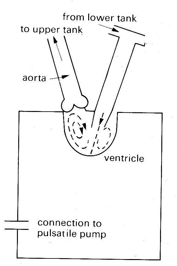
Fig. 11.30. Diagram of mode1 left ventricle showing diastolic flow patterns. (From Bellhouse (1972). The fluid mechanics of heart valves'. Cardiovascular fluid dynamics, p. 275. Academic Press, New York.
In model experiments it has been shown that the movement of the valve cusps towards each other is dependent on the strength of this vortex, and that regurgitation through the valve increases greatly if the vortex strength is reduced either by the delaying of ventricular contraction after the end of forward diastolic flow so that the vortex dies away, or by greatly increasing the size of the model ventricle so that only a very weak vortex is formed.
The mechanical reasons why the valve begins to close while there is still forward flow through it can be understood quite simply. We refer to Fig. 11.31,
Fig. 11.31. Schematic representation of mitral valve orifice and left ventricle. Row through the valve from the left atrium during diastole occurs in the direction shown by the arrow, with velocity U. Vortices are set up behind the valve cusps.
which is a schematic representation of a ventricle in which the region occupied by the vortices is significantly larger than that enclosed between the valve cusps. During the approximately steady state of forward flow which exists before deceleration, the pressures on either side of the cusp, at the points marked P and Q for instance, are equal and the valve cusps are therefore stationary. When the pressure difference across the valve orifice causes the flow through it to decelerate, the larger size of the vortex regions, together with the inertia of the swirling fluid, means that the corresponding changes in the velocity of flow in these regions are smaller than those through the valve In consequence the pressure on the outside of the valve cusp, at P say, changes less rapidly than that on the inside, at Q. Roughly, we can say that the pressures between P and R on the outside of the cusps are unchanged, while there must be a pressure drop from R to Q on the inside to provide the observed deceleration. Therefore the pressure at P exceeds that at Q, and the valve will tend to close. It should be emphasized that this analysis is very rough and ignores many details of the motion which would influence the magnitude of the pressure differences across the valve cusps. However, it probably does describe the essential mechanism involved in valve closure.
Mechanics of aortic valve closure. The structure of the aortic valve has already been briefly described. It has three cusps, attached to a circular ring of fibrous tissue which forms the 'outflow tract' at the base of the left ventricle; each cusp has free margins right to the wall, and the valve can open without distortion to expose the full cross-sectional area of the outflow tract. Immediately behind each cusp of the valve is a rounded pouch in the aortic wall, known as a sinus of Valsalva; and off two of these open the left and right coronary arteries, which supply blood to the muscle of the heart wall itself. Each valve cusp is extremely thin (0.1 mm) and is composed largely of elastic tissue and collagen, covered with a layer of endothelium similar to that lining the arterial walls.
The anatomy of the pulmonary valve is very similar, the only significant difference being that there are no coronary arteries opening off the sinuses of Valsalva in the pulmonary artery. As we have seen, the absolute pressure within the pulmonary artery, and its time-course, both differ somewhat from those in the aorta, and the same is true of the amplitude and time-course of flow. In the mechanics of valve closure, these differences may or may not be important; to date the experimental work on models, and the very few visualization studies which have been carried out in vivo, all relate to the aortic valve, so that the description given here applies primarily to it.
Direct information about the behaviour of even the aortic valve is very scanty. Cine-angiography in normal animals and man certainly confirms that the aortic valve does not obstruct forward flow during systole, but does not reveal any detail of valve-cusp behaviour. In one or two high-speed cine studies of radio-opaque particles, circular motion in the sinuses of Valsalva has been reported, but the existence of a vortex mechanism controlling the movement of the aortic valve, although a very old idea, has had to be established largely by model studies. It has of course been clear for a long time that some mechanism controls the movements of the valve, since measurement of instantaneous flow in the proximal aorta (e.g. Fig. 11.5, bottom waveform) has consistently shown that less than 5 per cent of the stroke volume normally flows back into the ventricle during valve-closure. Furthermore some flow occurs into the coronary arteries during systole (Fig. 11.20), implying that the orifices of the coronary arteries are not occluded by the cusps of the aortic valve.
Studies of realistic models of the aortic valve region, both by direct visualization and by measurements of pressure and velocity distribution in unsteady flow, have established that a vortex is generated behind each cusp of the valve during systole. As the valve is swept open, the ridge at the downstream end of the sinus acts as a stagnation point, and flow is diverted from the main stream into the sinus, where a vortex is set up (Fig. 11.32).
Fig. 11.32. Streamlines in aortic root at peak systole. (From Bellhouse (1972). "The fluid mechanics of heart valves'. Cardiovascular fluid dynamics, p. 264. Academic Press, New York.)
This controls the position of the valve cusp so that it holds a stable position during acceleration and peak systolic flow, without either blocking the coronary arteries or obstructing forward flow. During flow deceleration the valve cusps move evenly towards closure, and finally shut with very little leakage backwards at the end of the systole, as in the case of the mitral valve. When the experiments were repeated with a model in which the sinuses were not present, and the tube downstream of the valve was a simple cylinder, the valve became much less efficient, closing irregularly and late, with a good deal of backward leakage.
An approximate theoretical analysis of the operation of the aortic valve has been made by Bellhouse.* [* Bellhouse, B. J. (1972). 'The fluid mechanics of heart valves'. Chapter 8 in Cardiovascular Fluid Dynamics, ed. D. H. Bergel, Academic Press.] It involves two important assumptions. The first is that the effects of viscosity can be neglected, so that pressures can be related simply to local velocities and accelerations (as in Bernoulli's theorem, Equation (4.6)). This is justified because the whole cardiac cycle takes less than one second, whereas the time for viscosity to cause the flow in the vortex to decay significantly is about 20 s. The second assumption is that velocities within the vortex (i.e. its strength) are directly proportional to the aortic velocity just downstream of the sinuses of Valsalva. This assumption is not at all easy to justify, especially in the unsteady state during valve closure, when the flow is observed to spread out rapidly behind the closing cusps (Fig. 11.33).
Fig. 11.33. Streamlines during valve closure. (From Bellhouse and Talbot (1969). 'The fluid mechanics of the aortic valve',.J..Fluid Mech. 35, 721.)
Some of it goes to filling the expanding cavity behind the valve, and maintaining the vortex there, and the rest generates a very smooth flow downstream in the aorta. If, however, this assumption is accepted, then the mechanism of valve closure can be shown to be very similar to that already described for the mitral valve. Certainly, a theoretical analysis of the closure, which uses the observed time-dependent flow-rate through the valve, and the observed rate of closure of the valve, to predict local pressures in the aorta and the sinuses, gives results which correlate very well with those measured in the model. The great stability of cusp position during the accelerating part of systole can also be explained quite simply if a further assumption is made. This is that the strength of the vortex varies with the size of the region behind the cusp in the sinus. If the cusp is displaced so that it protrudes farther into the sinus than normally (Fig. 11.32), the strength of the vortex goes down. This means that the pressure there goes up, from Bernoulli's theorem, and hence tends to push the cusp back into its equilibrium position. The same argument works in reverse if the cusp is displaced outwards. Although the theoretical analysis of the motion of a valve cusp is based on important assumptions which cannot readily be justified a priori, the function of the vortex in the control of cusp-position seems clearly established.
Ejection from the left ventricle. So far, we have said nothing about the pressures and flows which are generated in the aorta by left ventricular ejection. These will de dealt with at length in the next chapter, where it will become clear that aortic pressure and flow are strongly influenced by downstream conditions as well as upstream ones. Here we outline very briefly the link between ventricular ejection and aortic events in systole by considering the balance of forces acting on the blood in the ventricle.
The aortic valve opens as soon as the pressure in the ventricle exceeds that in the root of the aorta. Before that time the ventricle contracts isovolumically, but afterwards the volume of the left ventricle (and perhaps its shape) as well as the pressure in the blood in contact with its wall change with time. The force which causes the blood to be accelerated out into the aorta comes from the difference between the pressure generated by the contracting ventricular muscle and that in the aorta. Its magnitude is approximately given by
ejection force = (pv - pa) A, (11.3)
where pv is a pressure representative of that generated by the contraction of the ventricle, pa is the pressure at the root of the aorta, and A is the area of the orifice into the aorta.
The time-course and magnitude of the pressure difference between the left ventricle and the root of the aorta can be obtained from Fig. 12.13, which shows pressure waveforms measured simultaneously at the two sites with high precision pressure manometers. Early in systole, left ventricular pressure rises rapidly to exceed aortic pressure, and it is at this point that flow into the aorta starts. The blood continues to accelerate until about half-way through systole, when the pressure records cross again. Thereafter, aortic pressure exceeds ventricular pressure, and the force acting across the aortic orifice (Equation (11.3)) changes sign, and acts to decelerate the flow. The flow does not actually come to rest or reverse its direction until considerably later, because it takes a finite time for the inertia it acquired during the accelerative period of early systole to be overcome by the adverse pressure gradient. Thus pressure gradient and acceleration are 'in phase', but pressure gradient and flow velocity are not: the velocity lags behind the pressure gradient. When the flow does reverse direction, the aortic valve closes, and this is marked by the notch on the aortic pressure record in Fig. 12.13 (the dicrotic notch). Thereafter, of course there is no continuity between ventricle and aorta, and the force balance breaks down.
If we consider the period when the valve is open, however, and assume that the effect of viscosity is negligible (which is justified because there is insufficient time during systole for viscous boundary layers to develop and resist the motion significantly) then the force acting to cause ejection (Equation (11.3)) must be equal, at all times, to the sum of two terms:
(1) the rate at which momentum is carried out of the ventricle;
(2) the rate of change of momentum of the blood in the ventricle (This is simply Newton's second law of motion, expressed in terms of momentum; this form of the law is explained in Chapter 2, Equation (2.9).)
The first of these terms can be estimated by considering the blood ejected from the ventricle in a short time 8t (Fig. 11.34).
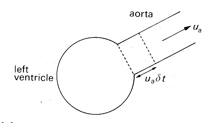
Fig. 11.34. Sketch of the left ventricle and aorta during systole. In a short time dt, blood in the aorta (moving with velocity ua will travel a distance ua dt.
Its mass is rAua dt where r is the density of the blood and ua is the instantaneous velocity of flow at the root of the aorta. The momentum (mass x velocity) of this blood is therefore (rAua dt)ua, which is the amount of momentum carried out of the ventricle in the time dt. Hence the rate at which momentum is carried out of the ventricle (this quantity divided by dt) is rAua2. This will vary continuously throughout systole.
The second term arises because the momentum of the blood remaining in the ventricle is also changing continuously. This momentum is equal to the sum of the momenta of all the elements of blood in the ventricle moving towards the aorta. Although it can only be calculated exactly if we know the shape of the ventricle and its rate of change of volume throughout ejection, we can predict that it will be equal to the mass of blood in the ventricle (pV, where V is the instantaneous ventricular volume) times the velocity of ejection (ua) times a scaling factor which we shall call I. Thus the rate of change of momentum in the ventricle is d(IrVua)/dt. If the shape of the ventricle did not change during contraction, I would be a constant. Since ventricular shape does change it probably varies, but in either case it can in principle be calculated.
Thus we can derive the following relationship, which will hold at all times when the aortic valve is open:
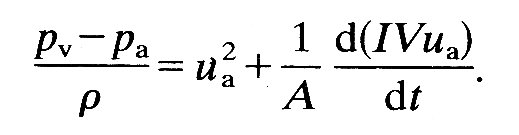 (11.4)
There is a further, more obvious relationship between ventricular volume V and aortic velocity ua; since blood is incompressible the rate of outflow into the aorta must be equal to the rate at which ventricular volume changes; i.e.:
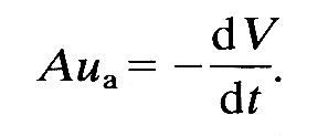 (11.5)
It is these equations which link pressure and volume in the ventricle to pressure and blood velocity in the aorta, and in principle they provide a means of examining ventricular performance from measurements in the aorta. If, for example, we know I and A, then systolic pressures and volume changes in the ventricle could be inferred from velocity and pressure measurements in the aorta, which are becoming practicable even in man by catheter techniques. In practice, there are great difficulties. For example, the value of I has not been determined for any shape of ventricle, nor its variability in vivo explored; furthermore, total ventricular volume V cannot be obtained from Equation (11.5) without knowledge of end-diastolic volume, which is notoriously difficult to measure accurately. So far, this approach has not been explored either theoretically or experimentally.
Finally, it should be pointed out that this description deals only with the forces relating to the motion of blood out of the ventricle, and ignores the very high pressure (aortic diastolic pressure) which the ventricle must overcome to open the aortic valve and initiate the motion. In a consideration of the overall mechanical performance of the ventricle, this latter term dominates. We can see this from Fig. 12.13 (§12.2.2); the excess pressure which the ventricle generates over that in the aorta is very small compared with the absolute level of the pressures.
11.5.3 Sounds and murmurs in the heart Sounds. There has been agreement for many years that the normal heart sounds are caused by closure of the valves. However, there has been sufficient confusion and misunderstanding about the basic mechanism to justify a detailed description.We will take the mitral valve, and therefore the first heart sound as an example. We have seen that at the end of diastole the valve-cusps are already close together; the last stage of closure is caused by retrograde flow of blood from the ventricle to the atrium. As the valve closes, the moving blood close to it continues in motion towards the atrium because of its inertia and stretches the valve. This is elastic, and therefore recoils, setting the blood in motion in the opposite direction. Again, therefore, the valve is carried past its equilibrium point and the process repeats itself. This oscillation continues until it is damped out by viscous energy losses in the blood and in the valve-cusps themselves
Of course the equilibrium position of the valve will be changing throughout this period, because the pressure difference across it is increasing as ventricular pressure rises. This will modify the process because the elastic properties of the valve-cusps are non-linear (stiffness increases with strain, as it does in arteries - and probably for the same reason; see Chapter 12). Nonetheless this is the basic mechanism which generates high-frequency pressure oscillations in the atrium and ventricle, and it is these which are the primary event in the generation of the first heart sound.
The misunderstandings about this mechanism which have arisen in the past appear to stem from two sources. First, the physical events have been misunderstood (for example, reversal of the pressure difference between atrium and ventricle has been assumed to cause instantaneous reversal of flow, which leads to mistiming because reversal is not instantaneous in a flow like this where inertia is important). Secondly, limitations in the performance of experimental equipment have caused events to be distorted or mistimed.* [* One example, which is particularly apposite here, is a form of distortion known as 'ringing' which may occur in pressure measurements with conventional catheter-manometer systems It consists of high frequency oscillations (which may be mistaken for events within the ventrical) and is caused by exactly the same mechanism as the heart sounds themselves. There is an elastic membrane (the manometer diaphragm plus the catheter walls) coupled to a mass (the fluid in the catheter), and when this mass is set in motion by a sudden change in pressure at the catheter-tip the diaphragm is displaced, overshoots, and the system oscillates briefly. Damping is again supplied by the viscous properties of the fluid.] The best proof that vibration of the valve is the origin of the heart sound comes from simultaneous recordings with paired microphones in the left atrium and left ventricle; these show that the vibrations which constitute the first sound are of opposite phase m the two chambers. An oscillatory motion of the valve seems the only way to interpret this fact.
All this does not mean that other events do not make any contribution to the heart sounds. The pressure fluctuations in the blood will set the heart walls in motion, and elastic waves will propagate over them (and along the arteries in the case of the aortic and pulmonary valves) in the manner described in Chapter 12. The sum of all these vibrations will contain components covering a wide frequency range. The higher frequencies (above about 50 Hz) will be picked up by the stethoscope if they reach the surface of the chest, and by high fidelity devices such as catheter-tip pressure transducers and catheter-mounted microphones. The low-frequency components (up to perhaps 20-30 Hz) can be picked up by conventional catheters and pressure transducers. If we take closure of the aortic valve as an example, the low-frequency vibrations register on aortic pressure recordings and are called the dicrotic notch (Fig. 11.5); the high-frequency vibrations are audible at the chest wall with a stethoscope and form the aortic component of the second heart sound. A pulmonary component occurs in the same way, but slightly later because right ventricular ejection lasts longer than left (Figs 11.5 and 11.6).
Considering their clinical importance, very little is known about the mode of propagation of the heart sounds. It should be made clear at once that in a true acoustic sense, they are not sounds at all. Acoustic sound waves are compression waves which travel within a material itself, accompanied by density changes; in liquids they have a very high velocity (about 1500 m s-1 in blood). Vibrations picked up at the chest wall by the diaphragm or bell of a stethoscope induce this type of wave in the air within the stethoscope tubing, and thus reach the ear as true sound; but the vibrations do not travel from their site of origin to the chest wall in this form. It has been shown that the heart sounds propagate along blood vessels like the aorta and through the tissues to the chest wall at velocities less than a hundredth of the acoustic sound-speed for blood; in the aorta, for example, the second sound travels at the velocity of the pulse wave (about 5-10 m s-1), and is rapidly damped out (i.e. 'stopped') if the vessel wall is locally bound so that it cannot move radially. Thus the second heart sound travels as a pressure wave in an elastic vessel exactly like the pulse-wave, and is in fact part of it, though its constituent frequencies lie outside those normally registered by pressure transducers. It is attenuated very rapidly as it passes along the vessel; virtually nothing is detectable 20 cm or more from the valve.
The first heart sound (i.e. pressure fluctuations set up by closure of the mitral valve) has been shown to spread over the ventricular wall in exactly the same fashion, moving towards the apex and then reflecting back at similar velocities, and in the same form, as the pressure waves in arteries described in Chapter 12. Finally, it has been shown that both heart sounds can travel either upstream or downstream from their point of origin. Thus the first heart sound from the mitral valve travels through the left atrium as well as the left ventricle, and the aortic second sound travels along the left ventricular wall as well as the aorta. How quickly the waves die out depends both on their frequency and on the stiffness of the wall along which they are travelling; they are damped out in a shorter distance when they travel through a relatively 'floppy' wall, or when their frequency is high.
These effects of frequency and wall-stiffness on attenuation are linked through the wave-speed. The frequency dependence is relatively simple to understand, because this type of wave attenuates by a given amount per wavelength (see Chapter 12); thus the higher frequency (shorter wavelength) waves will die out in travelling a shorter distance (and this will also take a shorter time). If, for example, a wave was travelling along the aorta, or back and forth over the ventricular wall, it might have a wave-speed of 5 m s-1, and attenuate by 50 per cent per wavelength. Then its amplitude would fall by about 97 per cent after travelling 5 wavelengths; for a wave at 100 Hz, this would be 25 cm, and would take 50 ms. For a wave at 50 Hz, both distance and time would be doubled. Thus if the vibrations are set up by a transient event like a valve closure, the higher-frequency components will fall off rapidly whether the waves are observed locally, decaying as they reflect back and forth, or followed along some particular pathway such as the aorta.
The effect of wall-stiffness on attenuation arises because the wave-speed is dependent on wall-stiffness (see Chapter 12), and falls as the wall becomes floppier; thus in a floppy tube the wavelength of our 100 Hz wave shortens, and it attenuates in a shorter distance (but not in a shorter time) than before.
When we leave the vascular structures themselves, and come to consider the mode of transmission of these waves to the chest wall, the situation is much less well understood. It is presumed that they induce vibrations in the chest wall either by direct contact, or via other interposed structures. Careful 'mapping' over the chest wall with multiple microphones has shown that each heart sound is detectable first at a particular site (which corresponds well in each case with the classical clinical site for listening with a stethoscope) and then radiates out over the chest wall, attenuating rapidly. The velocity of spread is again much too slow for a true sound wave, and high frequencies within the wave are attenuated much more rapidly than low; but beyond these facts, the physical nature of the wave has not been elucidated.
Murmurs. Most of the foregoing considerations apply also to the vibrations which correspond to audible murmurs, in the sense that they travel relatively slowly through the structures of the chest, primarily appear at particular sites on the chest wall, and show rapid attenuation of high-frequency components as they spread. Whereas, however, the origin of the heart sounds in vibrations of the valves is well established, there has been considerable uncertainty about the physical source of murmurs. The classical view has always been that they originated in the pressure fluctuations accompanying turbulence, and that the latter could occur in three main circumstances, when flow took place either through an abnormal valve, or through a normal valve when the chamber beyond was enlarged (jet formation), or finally where the anatomy was normal but there was a very high flow-rate across the valve. The extreme difficulties of visualizing flows in the heart satisfactorily, or of making direct measurements which would demonstrate turbulence, meant that most speculation about murmurs remained theoretical; and there are certainly other types of flow-disturbance which could act as a source of sound. The question of turbulence in the circulation will be dealt with in more detail when flow in large arteries is discussed (Chapter 12); for the moment it is sufficient to say that direct study of the frequency structure of murmurs, and of velocity fluctuations occurring in the blood in conjunction with them, makes it reasonably certain that murmurs do have their origin in turbulent disturbances. There remains, however, a great deal of uncertainty about the origins of other sounds coming from the heart in disease states; it is not at present possible to be really sure of the physical origin of third or fourth heart sounds, ejection clicks or the opening snap.
BERGEL, D. H. (1972) (ed). Cardiovascular fluid dynamics. Chapter 7: 'The meaning and measurement of myocardial contractility', by J. R. Blinks and B. R. Jewell; Chapter 8: 'The fluid mechanics of heart valves', by B. J. Bellhouse. Academic Press, London and New York. (2 vols).
CHALLICE, C. E. and VIRAGH, S. (1973) (eds). Ultrastructure in biological systems, Vol. 6: 'Ultrastructure of the mammalian heart'. Academic Press, London and New York.
CIBA FOUNDATION SYMPOSIUM (1974). New Series No. 24. The physiological basis of Starling's law of the heart. Associated Scientific Publishers, Amsterdam.
FUNG, Y. C., PERRONE, N, and ANLIKER, M. (1972) (eds). Biomechanics: its foundations and objectives. Chapter 12: 'Mechanics of contraction in the intact heart', by J. W. Covell; Chapter 13: 'Determinants of cardiac performance', by C. Urschel and E. H. Sonnenblick. Prentice-Hall, New Jersey.
HAMILTON, W. F. (1962) (ed.). Handbook of physiology. Section 2: 'Circulation', Vol. 1: several chapters on different aspects of cardiac physiology. American Physiological Society, Washington, D.C.
HILL, A. V. (1970). First and last experiments in muscle mechanics. Cambridge University Press.
TAYLOR, M. G. (1973). Haemodynamics. Ann. Rev. Physiol. 35, 87-116.