The term 'mass transfer' or 'mass transport' encompasses a vast range of processes involving the movement of matter within a system. It is not possible to provide a simple definition of its scope except to state that we are concerned with the movement of particular molecular species within a system and with the factors which affect the movement. We can introduce the subject by means of two simple examples, although these in no way describe its full breadth.
A puddle of water on the road surface slowly evaporates, the liquid water progressively being transferred as vapour to the air above it. The rate of evaporation depends upon such factors as humidity, the ambient air temperature relative to the ground, and the speed of the wind over the surface of the puddle.
If a crystal of copper sulphate is dropped into a beaker of water it slowly dissolves in the water and produces a concentrated solution around the crystal surface. In time this dissolved material diffuses further and further into the surrounding water. The speed with which the crystal dissolves and the rate of transfer of dissolved copper sulphate to the bulk of the water phase can be modified by a number of factors. For example, the process would occur more quickly in hot water than cold, or if the beaker were stirred.
These examples illustrate the two most fundamental mechanisms of mass transport within a single medium (or phase), that is, diffusion and bulk motion or convection. They also illustrate the important class of phenomena - transport of substances across the interface between phases; here the gas-liquid and liquid-solid interfaces. In biological systems we often encounter the transport between two liquid phases separated by a membrane, for example the cell membrane. Such transport can be by bulk motion and by diffusion, the details depending on the structural and chemical properties of the membrane and factors such as concentrations and pressures within the phases. In this chapter we will show how simple mass transfer processes may be examined quantitatively and estimates obtained of the behaviour of more complicated systems.
It is necessary to begin with some definitions. The first quantity to consider is concentration, which may be defined in various ways, in particular as mass concentration, mass fraction, molar concentration, and mole fraction (see Chapter 3, §3.4 for a definition of a mole). All are equally admissible, but, since we are concerned mainly with transfer between and within the liquid and solid phases we will use molar concentration. The molar concentration cA of species A in a solution is defined as the number of moles of A per unit volume and is usually expressed in the units g-mol l-1. If we now measure the amount of material A moving in a given direction, we may define its molar flux J as the number of moles per unit time passing through a plane of unit area at right angles to its path. Molar fluxes are usually expressed in the units mol s~1 cm-2. The definition of flux involves specification of the direction in which the movement is measured; a flux is a vector quantity and we must always be aware of this.
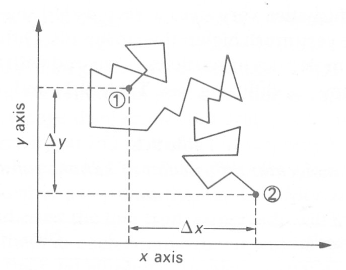
In 1827 the Scottish botanist Robert Brown performed a very simple but important experiment which led to a deeper understanding of the behaviour of molecules in a liquid. Brown discovered that grains of pollen on water moved about ceaselessly in a random manner in all directions (Fig. 9.1).
Fig. 9.1. Illustration of Brownian motion of a small particle on the surface of a liquid. Each line represents an individual motion. After some time the particle initially at station 1 has moved to station 2. Dx and Dy represent the projected displacements in the x- and y-directions.
This completely random or erratic motion of the pollen grains has subsequently been observed with small suspended particles of all kinds and is now termed Brownian motion. The motion of these particles is caused by the motion of the molecules of the liquid in which the particles are immersed. The molecules are in a continual state of random motion and as a result they continuously collide with one another and the suspended particles. The haphazard movement of the particles reflects this random molecular movement; whilst the individual molecules and their displacements are too small to observe directly, the consequential motion of the particles can be seen. The displacement of the particles results from the impact of a very large number of molecules at any instant of time.
The motions of the molecules of the liquid reflect their kinetic energy, which increases with temperature. As would be expected, the displacements of the particles also increase with temperature. The particle motion will depend also upon the viscosity of the liquid, the displacements decreasing as the viscosity of the medium is raised.
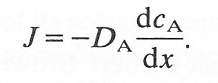
In 1855, Adolf Fick, the German physiologist (whose name is given also to the dilution method for determining cardiac output), formulated his famous law of mass transfer. This states that whenever there is a variation in concentration of any material (A) within a medium, there is a flux (J) of A in the direction of diminishing concentration (x-direction) and this flux is proportional to the concentration gradient (dcA/dx). Thus
 (9.1)
(9.1)
The constant DA is called the diffusivity or diffusion coefficient of the material. This equation has been shown experimentally to be applicable to the diffusion of both molecular and particulate material when in low concentration (see §9.3).
The values of diffusivities vary over a very wide range; typical values for diffusion in gases are very much higher than in liquids. Diffusivities also depend upon the size of the molecules or particles compared with the molecules of the medium in which they are diffusing (see Table 9.1)
Table 9.1 Comparison of molecular diffusivities of various substances at room temperature |
|
| species | diffusivity |
|---|---|
| O2 in air | 0.21 cm2s-1 |
| H2 in air | 0.41 cm2s-1 |
| O2 in watter | 1.8x10⁻⁵ cm2s-1 |
| H2 in water | 5.1x10⁻⁵ cm2s-1 |
| Acetate in water | 0.8x10⁻⁵ cm2s-1 |
| Low-density lipoprotein in water | 10-7 - 10-8 cm2s-1 |
and, like the intensity of Brownian motion, upon the temperature. It can be shown* [*This assumes that the molecules do not change shape or size as temperature changes; thus factors such as alteration in the degree of hydration are not included.] that if the absolute temperature of the medium is T, then
D=kT/m,
where m is the fluid viscosity (which also depends on temperature) and k a constant dependent upon the molecular characteristics of the medium. At first sight it would appear difficult to relate the random motion of the pollen grains in Brown's experiments to the formal law of Fick. However, it is possible to demonstrate a relation between the probable displacement (Dx) of a particle or molecule in a given time to the diffusivity D of that material. Imagine a water surface with pollen grains floating on it and undergoing Brownian motion over the surface. Consider a rectangle ABCD drawn in the surface with a line PQ bisecting it (Fig. 9.2) so that the lines AB and CD are
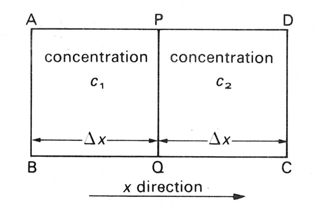
Fig. 9.2. Rectangular area of surface; see text for details.
each a distance Dx from the line PQ. We wish to compute the number of pollen grains which will cross the line PQ from either side during a small time interval. The concentration of pollen grains in the rectangle ABQP is c1 (the concentration is defined here as the number of grains per unit area); the concentration in CDPQ is c2. If the average displacement of grains is Dx in a time interval of t then the particles arriving at PQ from the left can only be those whose initial position is at AB or closer to PQ. Similarly particles crossing PQ from the right were originally no further away than the line CD. Moreover, only half of the particles which could cross the line from either side will in fact do so because, on average, half of them in each compartment will be moving away from PQ not towards it. Thus the total number of particles moving to the right across the line PQ is given by
number = 1/2 x area ABQP x local concentration
= 1/2 c1 x area ABQP.
Similarly the total number moving to the left is given by
number = 1/2 c2 x area CDPQ.
Hence the net number of grains moving from left to right in time t
= 1/2 c1 x area ABQP - 1/2 c2 x area CDPQ
= 1/2 (c1 - c2) x a Dx,
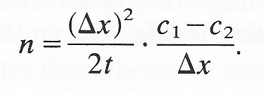
where a = length of the lines AB and CD. The net flux n (number of particles per unit time and unit length of PQ) is given by
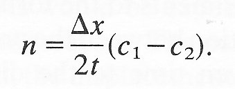
If we multiply top and bottom of the right-hand side of this equation by Dx,
But if we consider concentration changes over a small distance,
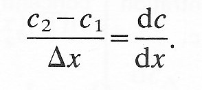
Thus
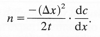 (9.2)
(9.2)
Comparing Equation (9.2) with the mathematical expression of Pick's law (Equation (9.1)) we can see that
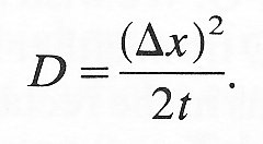 (9.3)
(9.3)
Thus the diffusion coefficient and the probable distance travelled by a particle or molecule in a given time are directly related.
While Fick appreciated that the driving force for diffusion was derived from the kinetic energy of the molecules, he was unaware of any physical significance of the diffusion coefficient. It was later shown by Nernst that if the molecules are assumed to be spherical, the diffusion coefficient is related to the frictional forces operating on them thus:
D = RT/fN (9.4)
where R is the Universal Gas Constant, T is the absolute temperature, N is Avogadro's number (the number of molecules per mole), and f is the frictional force opposing the motion of a molecule. If the diffusing molecule, is large compared with its surrounding molecules, then Stokes' law (Equation (6.1), §6.3) may be used to describe the frictional force:
f = 6pma (9.5)
where m is the fluid viscosity and a is the 'effective' radius of the molecule - commonly called the Stokes-Einstein Radius. This is not the actual radius of the molecule, but the radius of an equivalent spherical molecule, exhibiting the same diffusivity. Equations (9.4) and (9.5) can be combined to give an expression for a:
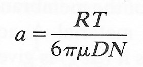 (9.6)
(9.6)
Thus this radius can be determined from a measurement of the diffusivity in free solution.
In the discussion so far we have implicitly assumed that the concentration of the diffusing species is low and the solution is said to be dilute. The diffusing molecules are considered to move about and interact only with the molecules of the carrier fluid. However, as the concentration increases so do the molecular interactions of the diffusing material. The effect of these interactions is to decrease the activity of the molecules and hence the diffusivity to some degree. A discussion of the detailed mechanism by which this happens and any indication of the magnitude of the effect are both beyond the scope of this book; the reader should simply be aware of the effect and its possible importance in situations where mass transfer is occurring in concentrated solutions.
A precise definition of this state is difficult and is not necessary for our purposes. Colloidal solutions, or sols as they are generally known, may be solutions of either very large molecules or aggregates of smaller molecules. The distinction between a sol and a particulate suspension (or an emulsion, which is a suspension of liquid droplets) is arbitrarily made according to whether or not the solute molecules or particles are visible under a light microscope (in a sol they are not).
It is often found that the individual large molecules of a sol are not in 'simple' solution but that solvent molecules are adsorbed on to their surfaces, resulting in complexes much bigger than the original molecule. The tendency for large molecules to imbibe water depends upon the electric charge distribution on the surface of the molecules and on the pH of the environment. Progressive removal of the free solvent from a sol ultimately causes it to solidify into a gel. When this happens the absorbed solvent remains trapped within the solid matrix, and if removed causes destruction of the gel structure.
As can be imagined, sols are common in biological systems, for example in the interstitial space between cells (see §13.2.5). This space contains various large molecules which have a very great affinity for water and as a result are considered to be present in colloidal solution.
In many practical situations, particularly in biology, it is not convenient and indeed often not possible to consider transport rates simply in terms of the molecular diffusivity. This is particularly true when we have to consider diffusion through cell membranes, as we often know neither the effective area for diffusion nor the thickness of the membrane. To overcome such difficulties we state that the flux (J) of material A across a membrane for a given concentration difference across it (DcA) is given by
J = KDcA (9.7)
where we define K as the mass transfer coefficient. Thus all diffusion pathways are lumped together and assessed by the one overall coefficient. The resistance of the membrane is then defined as 1/K.
In many biological situations diffusion occurs through a series of cell membranes and liquid layers. Let us consider an example with three layers as shown schematically in Fig. 9.3.
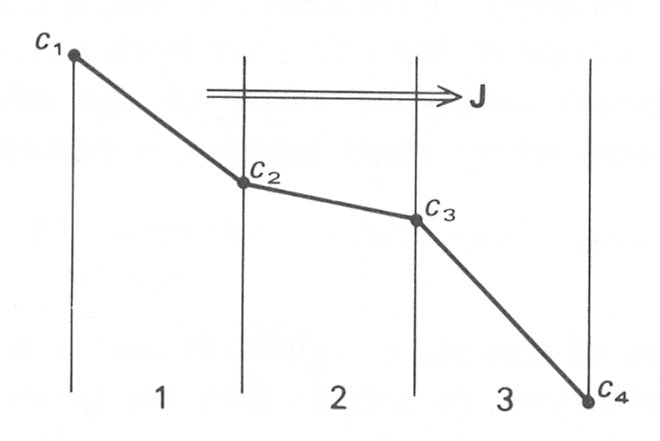
Fig. 9.3. A schematic representation of a three-compartment membrane showing the concentration profile across it under steady state conditions.
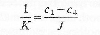
The overall concentration difference across the composite system is c1 - c4, but the distribution of concentration within the membranes is not a simple linear function of position, depending rather upon the relative mass transfer coefficients of the three sections. At steady state we know that the flux (J) through all three zones must be the same. Then applying Equation (9.7) to each of the three zones we have
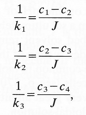
where k1, k2, k3, are the mass transfer coefficients for the three zones. If we add these three equations together,
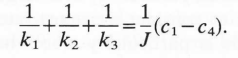
We may define an overall mass transfer coefficient (K) for the composite membrane on the basis of the overall concentration difference
Thus we can see that
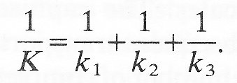
Since 1/k1 is the resistance of zone 1, etc. we see that the overall resistance to transfer is the sum of all the component resistances. Furthermore if one of the component resistances is very large compared with the others, then the overall resistance and the overall mass transfer rate will be determined by the transfer across that section. The difference in concentration across that section will be close to the overall concentration difference and that section of the membrane will be said to be the rate controlling section.
In later chapters we shall be concerned with the diffusional transport of molecules across the walls of blood vessels. This is very complicated and here only a simple introduction is provided to diffusion and nitration through pores and membranes. We shall consider first some very elementary aspects of the process and then restricted or hindered diffusion.
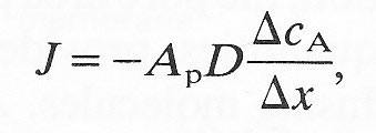
Consider a container filled with a solution of a substance at a concentration c1 separated from a second container by a porous filter of area Am, the second container being filled with a similar solution but of concentration c2. The concentration gradient existing because of the difference in concentration on the two surfaces of the filter will allow a diffusional flux of solute, from the container of high concentration to the other, with counter diffusion of the solvent. Provided the pore diameter of the filter is very large compared with the size of the solute molecules we may readily compute the flux on the basis of Equation (9.1); the effective area for diffusion is the pore area of the filter. The porosity of the filter is the pore area per unit area of filter or membrane (Ap) and Equation (9.1) may be written as
 (9.8)
(9.8)
where J is still the flux per unit area of filter and DcA is the concentration difference across the filter of thickness Dx.
If the filter is exchanged for others of the same porosity but successively smaller pore diameter, the flux of solute will at first be unaltered. However, beyond a certain critical size the pores will be too small to let the solute molecules pass through, and the flux will reduce to zero; smaller molecules than the solute can still pass through unimpeded, and are said to be sieved off.
This is the mechanism underlying the process of dialysis in which a membrane separates a solution of both large and small molecules from pure solvent. The passage of the large molecules is prevented but the smaller solute molecules can still pass through the membrane leaving the original solution relatively rich in large molecules. The capture of solute molecules by the membrane surface and the subsequent transport through it and release on the other side may depend upon a number of complex changes in the orientation of the molecules comprising the membrane. There are a number of molecular 'models' of biological membranes designed to describe different properties of membrane transport phenomena; none are yet fully agreed upon and we shall not discuss this subject further.
9.4.1 Restricted diffusion. The arguments presented in the previous section are really only applicable to diffusion through porous niters and membranes in which the pore diameter is many times the diameter of the solute or solvent molecules. It is not true to say that diffusion of molecules occurs unhindered till the molecules are as big as the pore. When the pore size becomes comparable with the random thermal displacements of the molecules, diffusion becomes restricted both because of collisions between the molecules and the pore edge and because of short range electrical forces between the molecules and the wall. Thus the effective pore area (As) available for transport decreases to zero as the molecular size increases.
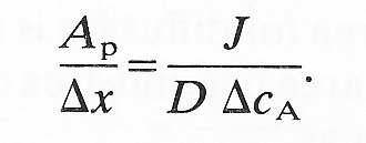
Many of the molecules involved in diffusional transport through biological membranes are comparable to the size of the water-filled pores through which they pass. Thus a pore of 4 nm radius will restrict the diffusion of glucose (radius 0.37 nm) compared with its free diffusion by approximately 35 per cent; it will even restrict the diffusional transport of water (radius 0.15 nm) by about 15 per cent. In order to describe this process quantitatively let us first rearrange Equation (9.8) in the form
 (9.9)
(9.9)
The left-hand side of the equation, the pore area per unit path length, is given in terms of readily measurable quantities, provided individual pores are of far greater diameter than the diffusing molecules. As pore dimensions decrease there is a geometric hindrance for molecules entering the pore and also an increase in resistance to diffusion along it. As a result D should be replaced by DR (a restricted diffusion coefficient) and the true pore area Ap by an effective pore area As. Equation (9.9) may then be rewritten as
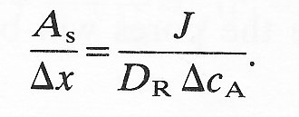 (9.10)
This gives an expression for DR in terms of the apparent pore area, and enables us to compute the flux of molecules through a membrane with small pores as long as As and Ap are known. The problems of doing this in practice are discussed in detail in Chapter 13.
Many biological and synthetic membranes also demonstrate the property of semi-permeability. This means that they are capable of selectively preventing the passage of some molecules and ions whilst permitting the passage of others.
The earliest explanation of semi-permeability was that the membrane acted simply as a sieve or porous filter, retaining the large molecules but allowing passage of the small ones. Whilst this mechanism is the basis of separation in filtration and in passive diffusion through membrane pores, it is now known not to be the sole cause of semi-permeability. It is possible for solvent molecules to pass through the membrane but for dissolved solute molecules to be prevented from passing through even though they may be smaller in diameter than the solvent molecules.
This apparently anomalous behaviour can result from a number of causes. For example, if the solute molecules have solvent molecules hydrated on to them, their effective size may be increased markedly; the solute molecules may also be aggregated. Electrical interactions between solute molecules and the pore walls may also prevent their passage.
Perfect semi-permeable membranes are capable of preventing the passage of the solute molecules completely; many membranes are not perfect and do allow some passage, and they are said to be 'leaky'. The cause of this leakiness can be either inherent in the membrane or the result of physical weakness of the membrane so that it breaks down or partially ruptures because of high pressure differentials set up across it by osmosis (see §9.7).
9.4.2 Active transport. Many biological membranes can transport materials faster than expected or against concentration differences by processes which require metabolic energy. This is called active transport, and is essential for the maintenance of the correct environment for cells. Many details of the mechanism are poorly understood, but the basic mechanism appears to be the same for all transported substances and to depend upon the existence of carriers within the membrane (Fig. 9.4).
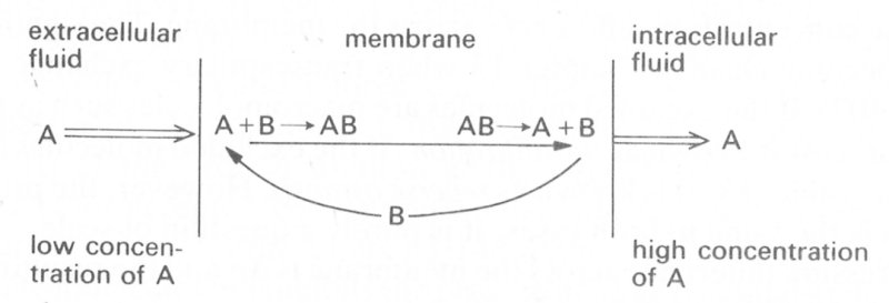
Fig. 9.4. A schematic view of a cell membrane showing the mechanism of active transport of molecules of A from outside to inside the cell. The carrier molecule B is retained within the membrane.
Molecules of substance A in the extracellular fluid are adsorbed on to the membrane and there combine with the carrier B to form the complex AB. This is then transported across the membrane, and at the intracellular side the complex is split and A is released to the inside of the cell. The carrier B then diffuses back to the outer surface of the membrane to combine with more A. Energy is consumed in the formation and breakdown of the chemical bonds in the membrane.
Because of the complexity of the structure and properties of biological membranes, it is usual to describe molecular transport through them in terms of their permeability. Thus if the flux of some solute (A) across the membrane is J when the concentration difference across the membrane for that solute is DcA, then
J = PA DcA (9.11)
where PA is the membrane permeability for solute (A). The coefficient (PA) in this equation is a mass transfer coefficient as defined above in Equation (9.7). The membrane permeability for any substance will depend upon many factors, in particular solute concentration and temperature, and it is important to report these whenever referring to a permeability. If concentration is not quoted, it is assumed that the solute is in dilute solution (see §9.3). Temperature has an important influence on permeability since it determines the amount of energy available to permit transport across the membrane. This is because energy is required for the solute to be adsorbed on to the membrane surface and to cause conformational changes in the molecular structure of the solute or membrane.
Thus far we have considered only diffusional transport through membranes. Transport can occur also by filtration through the pores if there is a pressure difference across the membrane, and this will be complementary to any diffusional transfer. A feature of this process is the ability of the mobile species to move independently of any concentration gradients if the pressure gradient is large enough. If the pores of the membrane are small enough to prevent passage of some of the constituents of the fluid, then the filtration process can itself cause concentration differences across the membrane. The significance of this will become clear in Chapter 13 when transcapillary exchange is considered (§13.7). If the excluded molecules are macromolecules such as proteins, then the process is known as ultrafiltration; if the excluded molecules are small such as inorganic salts it is known as reverse osmosis. However, the principle of operation is the same in both cases; it is purely a question of scale.
If the pressure difference across the membrane is Dp and the resulting flux of filtrate is J, then for simple membranes
J = F Dp (9.12)
where the constant F is called the filtration coefficient, analogous to the mass transfer coefficient in Equation (9.7). The nitration coefficient depends upon such factors as the number of pores per unit area, their size, shape, length and tortuosity. For a given geometry, F also decreases as the viscosity of the fluid is increased. Equation (9.12) could be derived theoretically if one assumed that flow within the pores obeyed Poiseuille's law, though the value of F could not be accurately predicted.
The phenomenon of osmosis (from the Greek word meaning 'to push') is of fundamental importance in all considerations of mass transfer in biological systems.
Imagine that a rigid porous filter separates two reservoirs as shown in Fig. 9.5.
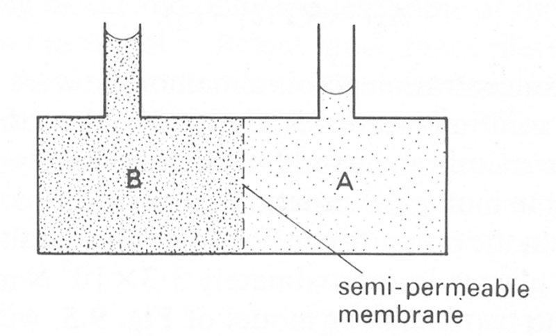
Fig. 9.5. Schematic view of two chambers A and B separated by a rigid semi-permeable membrane. Compartment B contains an aqueous solution of protein, compartment A contains no protein.
If an aqueous protein solution is introduced into chamber B and chamber A is filled with water, then a concentration difference for the protein is established across the barrier. However, if the pore size of the filter is sufficiently small, then protein molecules will be unable to diffuse through the barrier into chamber A. The water in chamber A will, however, diffuse into chamber B, reducing the concentration difference. As a result there will be an increase in the volume of fluid in chamber B.
If both chambers have tubes let into the top as shown in Fig. 9.5, then the liquid level in B will rise as water diffuses into the chamber and that in A will fall. In time, the levels will cease to change, indicating that there is no further net flow of water. At this time an equilibrium has been achieved between the 'force' driving diffusion and a 'force' due to the excess hydrostatic pressure in the compartment. At equilibrium, this excess pressure is called the osmotic pressure (P) of the protein solution at the equilibrium concentration. The symbol P is an accepted convention and should not be confused with the mathematical symbol for the number 3.142. If the membrane allows passage of small solute molecules but inhibits the passage of large colloidal molecules then the osmotic pressure which is established is called the colloid osmotic pressure or oncotic pressure.
Thus we can see that osmosis occurs whenever two solutions of differing concentration are separated by a barrier which allows passage of solvent but not the solute; it can result either from separation due to diffusion or from separation during filtration.
It can be shown that the osmotic pressure of a dilute solution whose total molar solute concentration is c (i.e. c is the sum of the molar concentrations of all solute species) at a given absolute temperature T is given by van't Hoff's Law:
P = cRT (9.13)
where R is the Universal Gas Content = 8.31 N m K~1 mol-1. Thus the osmotic pressure difference (DP) across a membrane where the solute concentrations are c1 on one side and c2 on the other is given by
DP = RT (c1 - c2). (9.14)
If the difference in concentration across a membrane were 1 mol cm-3 and the temperature of the solutions were 25 °C (298 K), then the osmotic pressure difference across the membrane would be approximately 1360 atmospheres! Thus we can see that in biological situations, even where solute concentrations are fairly low, the osmotic pressure can be quite considerable; for example, the osmotic pressure of plasma is approximately 3.3 x 10³ N m-2 (25 mm Hg).
Consider again the two-chamber model of Fig. 9.5, with a piston inserted into the tube above chamber B. By applying a load to the piston it is possible to increase the hydrostatic pressure in the chamber. At some instant, let the concentration of protein in the chamber B be c1, then the osmotic pressure of the solution P1 is given by Equation (9.13); if a pressure p1 (equal in magnitude to P1) is applied to chamber B via the piston, then further passage of water into the chamber can be prevented and the protein solutions will not be further diluted. The osmotic transfer of water is stopped. This does not mean that water molecules do not cross the membrane, for they continue to diffuse across it in both directions; there is simply no net flux.
Van't Hoff's law is really only applicable to a perfect semipermeable membrane separating two solutions; if for any reason the membrane is leaky then the osmotic pressure difference is less than predicted by Equation (9.13). For instance, if two water-filled chambers are separated by a membrane with pores of 6 nm diameter, then the addition to one compartment of an ideal solute of the same molecular diameter as the pore diameter will generate an osmotic flow of water as given by van't Hoff's law. If, however, the same molar concentration of small molecule (say urea, diameter 0.5 nm) were added to one compartment instead of the large molecule, the resultant osmotic flow would be less than 5 per cent of that predicted because most of the small molecules would be able to diffuse through the membrane.
This led to the empirical modification of the law as
P = scRT (9.15)
where s is termed the osmotic reflection coefficient. Its value varies from one for a perfect semi-permeable membrane to less than zero when the mobility of the solute is greater than that of the solvent.
The relationship between the osmotic and hydrostatic pressures of a solution is very important in biological exchange processes since the transfer of molecules almost always involves a change in both pressures. Indeed, both capillary filtration and transcapillary exchange involve consideration of the interaction between these two processes and will be discussed in Chapter 13.
In the circulatory system we are concerned with the transport of materials between the flowing blood and body tissues. Some of the mass transfer occurs by nitration across the vessel walls but much takes place by diffusion around and through cells. As an introduction to the later discussion on mass transport within the circulatory system we must first consider theories and models which have been developed to describe some simple dynamic mass transfer processes.
Let us consider in detail what happens when a crystal of copper sulphate (material A, Fig. 9.6)
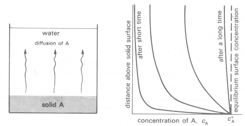
Fig. 9.6. The diffusion of a soluble material A into a stagnant liquid (e.g. copper sulphate into water) showing the progressively changing concentration profile with time in the bulk of the liquid.
is immersed in still water. Initially there will be no material A in the water phase, but after a short while, as A dissolves and diffuses away, the water close to the surface will contain A. In a thin layer very close to the crystal surface, the solution will rapidly become saturated in that no more molecules of A can be contained in it at that temperature. The concentration there is called the equilibrium surface concentration cA*, and at all times the concentration of A in this layer will be maintained at this level. Further away from the solid surface the concentration (cA) will be lower but will increase with time. Dissolution and diffusion away will continue to occur until the equilibrium surface concentration cA* is attained throughout the aqueous phase. Until that time, there will be a continuously changing concentration gradient (and hence flux) within the water as shown in Fig. 9.6. The decay in concentration with distance from the crystal surface will be roughly exponential and it is possible to determine how fast the concentration profile will change by applying Equation (9.3). For example, the distance (Dx) from the surface at which the concentration takes a particular value (e.g. 0.5 cA*) is directly proportional to (Dt)1/2. Thus material moves faster as D is increased and the distance travelled increases with the square root of time.
There are many situations where mass transfer occurs in the presence of bulk flow of material, and in such cases the transport rate is coupled to the flow conditions. An example is in blood vessels where we are particularly interested in mass transfer to and from the walls during flow. We must remember that the major resistance to transfer may be located in the wall rather than the blood and thus that the latter may not be very important in determining the overall rate of transfer. In order to understand the coupled effect of the flow and the diffusional exchange we will look at a very simplified model. Consider a long straight tube as shown in Fig. 9.7;
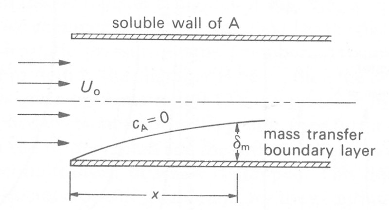
Fig. 9.7. A long tube with a slowly dissolving surface, through which steady laminar flow occurs. The growth of the mass transfer boundary layer is shown.
the flow entering the tube has a flat velocity profile which develops with distance along the tube as described in Chapter 5, §5.2. The wall of the tube is made of or contains a material which dissolves very slowly in the fluid, and fluid entering the tube contains none of this soluble material A. As the flow passes over the soluble section, then the wall progressively dissolves. Right at the beginning of the soluble wall (x = 0), the concentration of A in the fluid at the wall will be cA* (the equilibrium surface concentration) but there will be no A in the core of the fluid. As the flow proceeds downstream, diffusion of A away from the wall will occur and material will penetrate further into the core. However, because the core fluid is flowing downstream, the diffusing molecules will also be convected in that direction. If we map out the radial distance to which A will have diffused at progressive positions downstream (i.e. the distance from the wall to the points where cA becomes effectively zero as shown in Fig. 9.7) the line describes the surface of what is termed a mass transfer boundary layer (cf. the viscous boundary layer in Chapter 5).* [*In practice the local thickness (d) of the mass transfer boundary layer is defined as the distance from the wall where the local concentration of the species considered differs from its concentration in the core fluid by only 1 per cent of the total difference.]
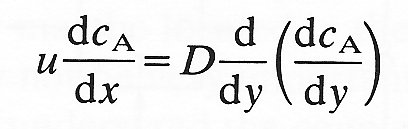
Once steady state conditions have been established we may calculate the approximate rate of growth of the mass transfer boundary layer with distance in a similar manner to the method used in Chapter 5 for calculating the growth of the viscous boundary layer. Consider a small cubic element of fluid within the boundary layer, as shown in Fig. 9.8,
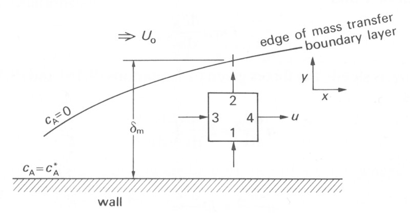
Fig. 9.8. A cubic element of fluid lying within a mass transfer boundary layer.
and let each face of the cube be of unit area. Then the diffusional flux into the bottom of the cube through face 1 will be given by Equation (9.1), based on the concentration gradient dcA/dy at the face. The diffusional flux out of the cube through the upper face 2 will also be given by Equation (9.1) using the concentration gradient across the upper face. Thus the net diffusional flux into the element is given by
net flux = diffusivity x rate of change of concentration gradient with y
or
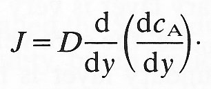 (9.16)
This is exactly analogous to the calculation of the net viscous stress on an element in the viscous boundary layer calculation of Chapter 5.
This diffusional flux into the element is balanced by the convection of the material downstream. The convective flux into the element through face 3 is
given by the concentration at the face multiplied by the velocity of flow into the element. We may compute the convective flux out through face 4 in a similar manner. Hence the net convective flux out of the element is given by
Flux = rate of change of (velocity x concentration) with x
or

Provided the rate of mass transfer is low and the molecules diffusing into the element do not contribute to a large change in its volume, then the velocity u is independent of x and
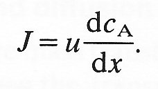 (9.17)
Since the flow is steady the fluxes given by Equations (9.16) and (9.17) must be equal. Thus
or
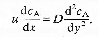 (9.18)
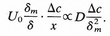
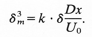
As was the case in computing the growth rate of the viscous boundary layer, we can most easily estimate the growth rate of the mass transfer boundary layer by ascribing suitable scales or magnitudes to each of the parameters in the equation. Thus at a distance x from the beginning of the soluble section, the mass transfer boundary layer thickness will be dm. Across the boundary layer at this location the concentration of A in the fluid falls from cA* at the wall to cA = 0 at dm from the wall and hence we can scale dcA as Dc where this equals (cA* - 0). The velocity scale within the mass transfer boundary layer will depend upon whether or not the viscous boundary layer thickness d is very much less than dm. If the viscous boundary layer is very much thinner, then the appropriate velocity scale will be U0, i.e. the core velocity of the fluid. On the other hand if the mass transfer boundary layer is much thinner than the viscous boundary layer, the velocity gradient can be assumed to be constant and a suitable velocity scale is U0(dm/d).
For the case where the viscous boundary layer is very much thinner than the mass transfer boundary layer we may substitute into Equation (9.18) as follows:
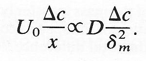
Then
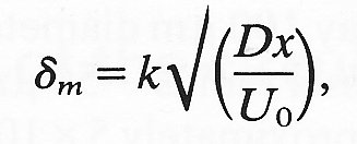 (9-19)
where k is a numerical constant whose size must be computed for any given situation. Thus the thickness of the layer increases with distance from the tube entrance as x1/2. If we compare this with Equation (5.3) (§5.3) they again appear very similar. Indeed we can see that
(d/dm)2 = n/D (9.20)
In the case where the viscous boundary layer is larger, substitution in (9.18) yields the relationship
Hence
If we consider the situation near the entrance of a tube, where d is given by Equation (5.3), we obtain
(d/dm)3 = n/D (9.21)
On the other hand, if we consider the case where the mass transfer is occurring in a section of the tube remote from the entrance in which the velocity profile has become established, then d is constant and
![]()
The boundary layer grows in thickness with distance along the soluble section as x1/3.
9.9.1 The Schmidt Number. The ratio n/D is a dimensionless quantity like the Reynolds number, and it is called the Schmidt number (Sc). Schmidt numbers for gases are typically about unity, but in liquids they are much larger. Thus for oxygen in water at room temperature, the Schmidt number is approximately 600; that for urea in water is 950 and lactose in water 2400. Typically in biological systems, Schmidt numbers for small molecules and ions (e.g. acetate) are of the order of 103; as the molecular size increases so does the Schmidt number. Thus large protein molecules can have Schmidt numbers of the order of 106 in water or plasma.
The enormous size of such Schmidt numbers has very great importance when we consider mass transfer processes in biological systems. If we calculate the expected thickness of the mass transfer boundary layer for a large protein molecule in a small vessel of say 100 mm diameter (the viscous boundary layer cannot be greater than the vessel radius - 50 mm), we can see from Equation (9.21) that the layer will be approximately 5 x 10⁻² mm or 50 nm thick. That is, it will be only a couple of molecules thick! Clearly the idea of a continuum breaks down under such circumstances but the calculation serves to indicate just how thin mass transfer boundary layers can be in biological situations.