When blood is ejected from the heart during systole, the pressure in the aorta and other large arteries rises, and then during diastole it falls again. The pressure rise is associated with outward motions of the walls, and they subsequently return because they are elastic. This process occurs during every cardiac cycle, and it can be seen that elements of the vessel walls oscillate cyclically, with a frequency of oscillation equal to that of the heart-beat. The blood, too, flows in a pulsatile manner, in response to the pulsatile pressure. In fact, as we shall see in Chapter 12, a pressure wave is propagated down the arterial tree. It is therefore appropriate in this chapter to consider the mechanics of pulsatile phenomena in general, and the propagation of waves in particular.
Let us examine first the oscillatory motion of a single particle. Suppose that the particle can be in equilibrium at a certain point, say P, but when it is disturbed from this position, it experiences a restoring force, tending to return it to P. There are many examples of this situation, as when a particle is hanging from a string and is displaced sideways (a simple pendulum), or when the string is elastic and the particle is pulled down below its equilibrium position. In cases like these, the restoring force increases as the distance by which the particle is displaced from P increases. In fact, for sufficiently small displacements, the restoring force is approximately proportional to the distance from P (see §8.5). If the particle is displaced and then released, it will return towards P, but will overshoot because of its inertia. The displacement will then increase in the opposite direction, so that the restoring force increases, slowing the particle down until it stops and then comes back towards P. Again it overshoots, and so on. The particle in fact oscillates about P.
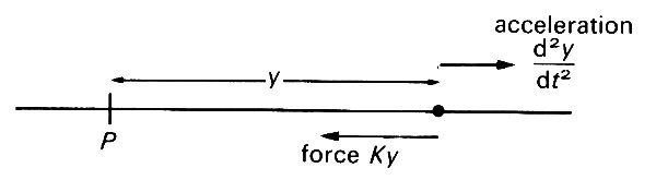
The mathematical analysis of this oscillation is very simple, and we give it here in full because we believe that it helps in gaining a complete understanding of the mechanics of oscillatory motion. Suppose the particle has mass m, and oscillates backwards and forwards in a straight line about its equilibrium position P (Fig. 8.1).
Fig. 8.1. A particle moving along a straight line under the action of a restoring force equal to K. times its displacement y from a position of equilibrium, P. Its acceleration from P is d2y/dt2. The equation governing its motion is (8.1).
If y is the distance of the particle from P, then the magnitude of the restoring force, directed towards P, is proportional to y, equal to Ky, say, where K is a positive constant, measured in appropriate units.
If we adhere to the convention that y should be considered positive for displacements to the right of P, and negative for displacements to the left, then the force on the particle in the positive y-direction is -Ky. Newton's law of motion states that this force is equal to the mass of the particle times its acceleration in the positive y-direction (this acceleration is equal to d2y/dt2: see Equation (2.5) §2.3). That is to say
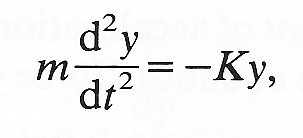 (8.1)
(8.1)
which can be rewritten
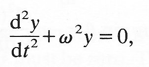 (8.2)
(8.2)
where w2 = K/m. Equation (8.2) is thus applicable to the oscillations of any particle about a position of equilibrium as long as the oscillations are small enough for the restoring force to be proportional to y. It represents a balance between the restoring force on the particle and its inertia; these two properties are essential for the presence of any oscillatory motion.
Perhaps the most common example is that of the simple pendulum, in which a particle (mass m) hangs almost vertically on a string of length l (Fig. 8.2).
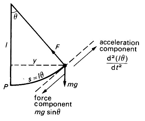
Fig. 8.2. A simple pendulum. The particle hangs on an inextensible string of length /, and oscillates in a vertical plane. The forces on the particle are its weight, mg vertically downwards, and the tension in the string, F. The most convenient direction for considering the force balance is perpendicular to the string; the components of force and acceleration in this direction are marked on the Figure and discussed in the text.
If we suppose the string to be inextensible, and if we neglect all air resistance and other frictional forces, then the only forces on the particle are its weight, equal to mg and directed vertically downwards, and a force F supplied by the string (the tension in the string), which is directed along the string. Since we do not know the value of F a priori, it is most convenient to consider the balance of forces in a direction at right angles to the string, because F has no component in this direction. If we let q be the angle which the string makes with the vertical (measured in radians), the only force acting in the given direction is a component of the weight of the particle, equal to mg sin q, and directed along the arc towards the equilibrium position (marked P on Fig. 8.2). The component of acceleration in the required direction is obtained by noticing that the particle is actually travelling along the circumference of a vertical circle, of radius l. The component of acceleration tangential to this circle is d2s/dt2, where s is the distance travelled along the circumference, measured from P. Thus s is equal to lq, and the tangential component of acceleration is d2(lq)/dt2 in the direction of increasing q (see Fig. 8.2). The equation 'force equals mass times acceleration' therefore gives
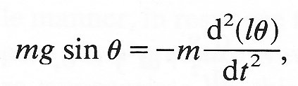
where the minus sign occurs because we want the component of acceleration in the direction of the force, not the opposite direction. This equation may be rewritten
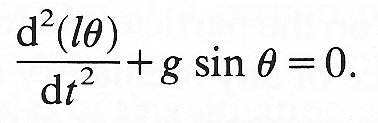
We notice that, if y is the horizontal displacement of the particle, then
sin q = y/L
Let us now suppose that q remains very small all the time; this means that the particle effectively oscillates along a horizontal straight line. It also means that sin q is approximately equal to q (see Chapter 7, §7.3), so that lq is approximately equal to y. In this case Equation (8.2a) reduces to Equation (8.2), with the quantity w2 equal to g/l.
In whatever manner the particle is released, its subsequent motion must be such that y varies with time in a manner consistent with Equation (8.2) for this particular w. (In mathematical terms, the function y(t) must be a solution of the differential Equation (8.2).) However, there is an infinite number of motions consistent with this equation; the particular one appropriate in a given situation is completely determined by the displacement y and velocity dy/dt at the time of release (we could, for example, release the particle from rest at a given displacement, or we could impel it away from P with a given velocity). The most general motion consistent with Equation (8.2) (its most general solution) is given by
y = A cos wt + B sin wt (8.3)
where A and B are any constants. The velocity of the particle, dy/dt, corresponding to this motion is obtained by differentiating Equation (8.3) with respect to time, and is
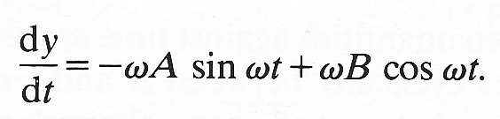 (8.4)
(8.4)
The values of the constants A and B may be determined from the initial values of y and dy/dt. As a first example let us consider a simple pendulum, whose bob (the particle) is pulled out a horizontal distance a from its equilibrium position, and released from rest there at the initial instant which we will call t = 0. That is, at time t = 0,
Now sin (0) = 0 and cos (0) = 1, so the second of these conditions, substituted into Equation (8.4), shows that B must be zero. The first condition, substituted into Equation (8.3), then gives A = a. Thus the solution of the problem, the complete motion of the particle for all time, is given by
y = a cos wt (8.5)
with velocity, again by differentiation,
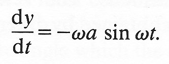 (8.6)
(8.6)
The graphs of these two quantities against time are shown on Fig. 8.3. It can be seen that y oscillates cyclically between a and -a, and dy/dt oscillates cyclically between +wa and -wa, and passes through zero when y is equal to either +a or -a. The quantity a is called the amplitude of the oscillation in position; wa is the velocity amplitude. The period of the oscillation, that is the time of one complete cycle, after which the motion reproduces itself exactly (marked T in Fig. 8.3),
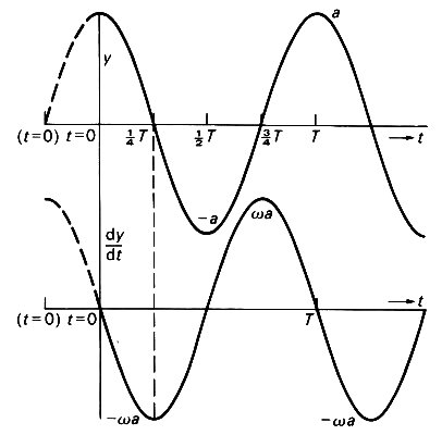
Fig. 8.3. Graphs of y and dy/dt against time when they are given by Equations (8.5) and (8.6). The amplitude of the oscillation in displacement is a, and that of the velocity is wa. The period of the oscillation is T ( = 2p/w). These graphs represent simple harmonic motion. The dotted extensions to the left, with a new origin, represent the graphs of y and dy/dt when they are given by Equations (8.7) and (8.8), with V = aw..
is equal to 2p/w.* [*This is a consequence of the trigonometrical definition of sine and cosine. Let us consider the quantities sin q and cos q as q takes values which increase from zero, with reference to Fig 8 4. In this figure is drawn a circle of unit radius centred on C, the origin of coordinates. The angle q is represented by the point A, so that the line CA makes an angle q with the x-axis. The coordinates ot A are (x y) Then sin q is defined in the right-angled triangle ABC as being the length of the opposite side AB divided by that of the hypotenuse CA. That is, sin q = y/1 = y. Similarly, cos q is defined as being the length of the adjacent side CB divided by that of the hypotenuse - cos q = x/1 = x. As x increases. sin q and cos q change accordingly, until when q exceeds the value p/2 radians (90o), the point A moves into the second quadrant, so that x is negative although y is still positive. Thus cos q is negative and sin q is positive for values of q between p/2 and p (180°). In the third quadrant, between p and 3p/2 (270°)), x and y are both negative and therefore so are cos q and sin q. In the fourth quadrant (q between 3p/2 and 2p (360°)), x is positive again, so that cos q is positive although sin q is still negative. If q is increased beyond 2p, the point A moves into the first quadrant once more, and everything starts again: cos q and sin q are both positive. We see that increasing the value of q by 2p, i.e. going around the origin once to get back to where we started does not alter the value of cos q or sin q. The 'period' of sin q or cos q is 2p. This explains why the distance between successive peaks of the graph of a cos wt (Fig. 8.3) is T=2p/w.]
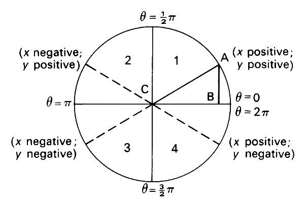
Fig. 8.4. Diagram to illustrate the periodic nature of sin q and cos q, as defined trigonometrically. In quadrant 1, both are positive; in 2, sin q is positive and cos q is negative; in 3, both are negative; in 4, sin q is negative and cos q positive. When q is increased by 2p (360°), sin q and cos q are unchanged. For further discussion, see footnote in §8.1.
The frequency f of the oscillation, i.e., the number of cycles or periods per unit time, is equal to w/2p; w itself (= 2pf) is called the angular frequency or radian frequency. (N.B. All frequencies have units of inverse time, s-1; this is because neither radians, the units of angle, nor the number of cycles have any dimension at all.) The quantities w and a are quite independent of each other; the frequency w is determined completely by the system under consideration (the mass of the particles m and the restoring force constant K), whereas the amplitude a is determined solely by the displacement and velocity at the time of release. It is interesting to note that in the case of the pendulum, the frequency is also independent of m, since w is equal to (g/l)1/2. The period of oscillation of a pendulum is thus independent of the mass of the bob; but for this, the operation and adjustment of a pendulum clock would not be as simple as it is.
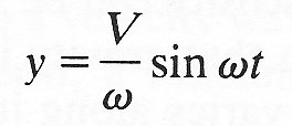
The solution corresponding to Equations (8.5) and (8.6) in the case when the bob of the pendulum starts off at its equilibrium position, but is given an initial velocity V, can also be written down simply. In that case, at time t = 0,
The first of these conditions, substituted in Equation (8.3), shows that A must be zero; the second, in Equation (8.4), shows that wB must be equal to V. The complete motion of the particle is then given by
 (8.7)
(8.7)
and
 (8.8)
(8.8)
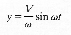
In this case, the amplitude of the oscillation in displacement is V/w; that in velocity is V. The angular frequency is of course still w. The graphs of these equations can be obtained from Fig. 8.3 by putting the origin of time a quarter period farther back (see the broken lines on that figure), and by replacing a everywhere by V/w.
Any motion described by Equation (8.2), of which those given by Equations (8.5) and (8.7) are particular examples, is called simple harmonic motion. Equation (8.3) represents the most general simple harmonic motion with the given angular frequency w; this can in fact be manipulated into the form
y = A' cos (wt - f) (8.9)
where A' = (A2 + B2)1/2 and f is an angle such that tan f = B/A. The amplitude of this oscillation is A'; f is called its phase, and the oscillation is said to have a phase lag of f behind an oscillation proportional to cos wt alone (Equation (8.5)). The graph of Equation (8.9) is given in Fig. 8.5,
Fig. 8.5. Graphs of Equations (8.9) (solid curve) and (8.9a) (broken curve). The solid curve has been shifted bodily to the right, by an amount corresponding to the time f/w; f is the phase lead of (8.9) over (8.9a).
and compared there with that of
y = A' cos wt (8.9a)
The graph has been shifted bodily to the right, as if the quantity wt had everywhere been diminished by an amount equal to f. In Equation (8.9a) everything happens at a time f/w earlier than in Equation (8.9), and the meaning of the phrase 'phase lag' becomes clear. If f is in fact negative, it is said to represent a phase lead. The quantity (-sin wt) in Equation (8.6) can be written cos (wt + p/2), so that the velocity of this oscillation has a phase lead of p/2 over the displacement. It can be seen from Fig. 8.3 that the graph of velocity reaches a given point in the oscillation (e.g. the minimum) at a time T/2 before the displacement graph, i.e. at a value of wt in advance by p/2.
From Fig. 8.3 we can retrieve all the details of simple harmonic motion: when the displacement y is a maximum, the velocity, dy/dt, is zero; the restoring force, however, is a maximum, and therefore so is the acceleration, directed back towards P (Fig. 8.2). As the particle returns towards P, y diminishes while the speed increases, until when it passes through P, where the displacement and acceleration are zero, the speed is a maximum. Beyond P, the speed diminishes again while the displacement and acceleration increase to their maximum values on the other side. The process continues indefinitely in the absence of friction.
The simple harmonic motion described above is a motion with one degree of freedom; it is completely specified by the determination of how one variable (the coordinate y of the particle) varies with time. A system with two particles on a string, one above the other, both of which can oscillate in the same direction (a double pendulum), or a system of one particle free to oscillate in a plane (like a pendulum whose string is elastic) has two degrees of freedom, since two coordinates are required to specify the motion. More general systems of particles have larger, but finite, numbers of degrees of freedom. On the other hand, in any continuous system, like a violin string, the water in a tank, or the walls of an artery, the coordinates of an infinite number of elements (e.g. fluid elements) must be specified for a complete description of the motion. Such a system therefore has an infinite number of degrees of freedom. The situation is not as complicated as it sounds, however, since all the elements are joined together, and in fact wave motions in continuous systems can be described quite simply.
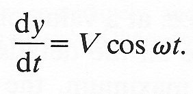
As a simple example, consider a stretched elastic string, fixed at each end, and suppose that at some initial instant it is plucked or struck or given a small sideways displacement in some other way, and then released (Fig. 8.6 (a)).
Fig. 8.6. If a stretched string, fixed at its ends, is displaced sideways as in (a), it will subsequently oscillate backwards and forwards, occupying a range of positions of which two are shown in (b) and (c). Such motion is a standing wave; the oscillation shown is the fundamental, with angular frequency w0 = (p/l)(F/M)1/2. In (d) and (e) are depicted the forms of two of the higher harmonics, with one and three intermediate nodes respectively, and with frequencies two and 4w0 respectively. A general oscillation consists of the superposition of many harmonics.
Again, we neglect all friction, and suppose that there is no energy dissipation by any means. The tension in the string provides a restoring force which tends to restore every displaced element to its equilibrium position (element AB, for example, clearly has a net downward force on it). Each element has mass, i.e. inertia, and therefore keeps moving until it has passed its equilibrium position; it is then slowed down by the restoring force, and subsequently executes simple harmonic motion as described above. At various times the string may look like Figs. 8.6 (b) or (c). This motion, in which the string is fixed at the ends and every particle executes simple harmonic motion, is called a standing wave. The frequency of the oscillations can be estimated by dimensional analysis. The only quantities it can depend on are the restoring force, provided by the tension F in the string, with units of force (kg m s~2); the inertia, supplied by the mass per unit length of the string M (units kg m-1); and the geometry, i.e. the length l of the string (units m). The only way to get a frequency (units s~1) from these three quantities is in the form {(F/M)1/2}/l, so the frequency must be proportional to this quantity. In fact, there is an infinite number of possible oscillation frequencies of a finite string fixed at its ends, which take the values a = {p(F/M)1/2}/l, {2p(F/M)1/2}/l, {3p(F/M)1/2}/l, etc., so although there is an infinite number of frequencies, they are separate from each other. They are called the natural frequencies of the string, in that however the string is disturbed initially, its subsequent motion will consist of the superposition of a number of oscillations each having one of the natural frequencies (see §8.6). The fundamental oscillation is that with frequency {p(F/M)1/2}/l; if the string moved with that frequency alone, it would oscillate backwards and forwards in the manner suggested by Fig. 8.6 (a), (b), and (c). An oscillation with a higher natural frequency is said to be a higher harmonic; the first harmonic, with frequency {2p(F/M)1/2}/l, oscillates in such a way that the mid-point of the string remains fixed (Fig. 8.6 (d)), at what is called a node. Subsequent harmonics have more fixed points or nodes (Fig. 8.6 (e)). An arbitrary oscillation, being a superposition of the fundamental and all its harmonics, will not generally have a node.
Now consider a string which is very long, and one element of it, say the element BC in Fig. 8.7 (a),
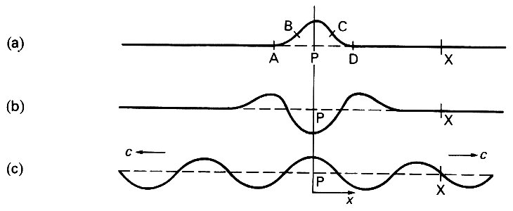
Fig. 8.7. Propagation of a travelling wave on an infinitely long stretched string. The point P (at x = 0) is forced to oscillate from side to side in simple harmonic motion. The initial displacement depicted in (a), causes the element BC to exert forces on elements AB, CD, tending to displace them. The element BC is returned towards equilibrium and overshoots. A little while later the string looks like (b). Later still it looks like (c), the disturbance propagating outwards with speed c.
is continuously made to perform simple harmonic motion with angular frequency w and some small amplitude a. Immediately after the start of the motion, the string will be deformed as shown in Fig. 8.7 (a). Because of the tension in the string, the element BC exerts a net upwards force on each of the neighbouring elements AB and CD, which begin to move upwards. They will still be moving upwards as the element BC begins to return towards its equilibrium position, and after a little while the situation will look something like Fig. 8.7 (b). The elements AB and CD then in turn cause displacement of the elements next to them, while themselves tending to be restored towards, and subsequently to overshoot, their equilibrium positions. This process is continuously repeated, and the oscillatory motion propagates along the string in the form of a travelling wave. Every element of the string executes simple harmonic motion, but elements progressively more distant from the origin P of the disturbance enter the oscillatory cycle at a progressively later time; that is, the phase of their oscillations lags increasingly behind that of the oscillation at P. The frequency and amplitude of the oscillations of every element will be the driving frequency w, and amplitude a. We can use dimensional analysis again to estimate the speed with which the wave is propagated in each direction along the string. The units of the wave-speed (which we may call c) are m s~1, and the only quantities on which it can depend are F, M, and w. There is only one way in which this can be done, and we see that c must be proportional to (F/M)1/2 (more precise calculations show that c is actually equal to (F/M)1/2, which is independent of the frequency w.
This is not the place to go through the mathematical derivation of wave-speed, etc., which is quite complicated, but we shall frequently wish to use the mathematical form of a travelling wave, and therefore set it down here. Consider a point X situated at a distance x to the right of P (Fig. 8.7), so that x is positive, and the wave will propagate past the point from left to right. At first there is no disturbance at X; the disturbance reaches X after a time ct, and, after the 'wave-front' has passed, the element of the string at X performs simple harmonic motion, with frequency w and amplitude a. Then the transverse displacement of the element at X, at time t (we shall call the displacement y) is given by
y = a cos {w(t - x/c)}* (8.10)
[*Equation (8.10) implies that y is zero, and dy/dt is equal to -wa, at the origin (P) at time t = 0. If this were not the case, either an adjustment would have to be made to the time we called t = 0, so that Equation (8.10) would be true, or a constant phase angle f would have to be inserted in the braces:
y = a cos {w{(t - x/c) - f}.
Then y = a cos f at x = 0 and t = 0.]
This equation represents a pattern of displacement which is travelling to the right with speed c. To see this, consider the graph of y against x at two successive times, t1 and t2 (Fig. 8.8).
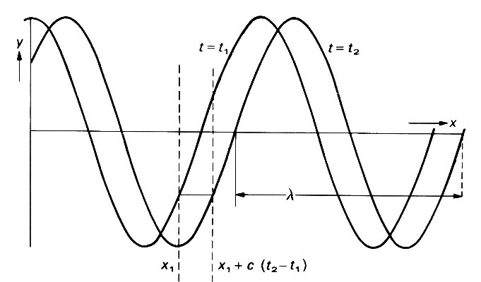
Fig. 8.8. Graphs of y against x, as given by Equation (8.10), and depicted at two successive times t1 and t2. The curve at time t2 has been shifted bodily to the right, by a distance c(t2 - t1); to see this notice that the value given by Equation (8.10) at position x1 and time t1 is the same as that given at position x1 + c(t2 - t1) and time t2. Thus the wave propagates with speed c. l is the wavelength.
At time t2, the displacement at position x = x1 + c(t2-t1) is the same, for any x1, as that at time t1 and position x1; this is because the quantity (t-x/c) has the same value, (t1 - x1/c), in each case. That is, the whole pattern has shifted a distance c(t2 - t1) to the right during the time interval t2-t1, and hence is travelling with speed c.
The wavelength l of the wave represented by Equation (8.8) or Fig. 8.8 is the spatial distance occupied by one complete oscillation. It is the distance travelled by the wave during one period of its oscillation. The period is 2p/w, so the wavelength, equal to the wave-speed times the period, is
l = 2pc/w (8.11)
As with simple harmonic motion of a single particle, the occurrence of waves requires the presence of both restoring force and inertia. In the above example, the restoring force is provided by the tension in the string, and the inertia by its mass per unit length. In the case of waves on the surface of a liquid (except for very short waves, where surface tension is important), the restoring force is gravity, and the inertia is provided by the density of the liquid.* Sound waves in a fluid are a balance between the density of the fluid and its compressibility, which causes any small local compression to spring back towards equilibrium. Pressure waves are also propagated along the elastic walls of arteries, where the restoring force comes from the elasticity of the walls, and the inertia is that of the blood within (and to some extent that of the wall itself); we show in Chapter 12 how the mechanics of blood flow in arteries can largely be described in terms of the propagation of such waves.
[*The speed of propagation c of surface waves on a deep, infinite ocean when surface tension is unimportant can depend only on the acceleration of gravity g, the density of the water r, and the wavelength of the waves l. By dimensional analysis, therefore, c must be proportional to (gl)1/2. Similarly, if surface tension dominates and if gravity is unimportant, c can depend only on r, l and s, the surface tension of the air-water interface, which has dimensions [MT-2]. In this case dimensional analysis shows that c must be proportional to (s/rl)1/2. Both gravity and surface tension will be important if these two estimates of the wave-speed are of similar magnitude, i.e. if the wavelength is approximately equal to the value lc where
lc = (s/rg)1/2
For an air-water interface, the value of s is approximately 0.07 kg s-2, so lc is approximately 0.002-0.003 m (2-3 mm). If the wavelength is much greater than lc, surface tension will be unimportant, and this is the case for most waves observed on the sea.]
All the oscillatory motions discussed above are governed by a balance between inertia and a restoring force, with no other forces acting on the particles involved. In such circumstances, the oscillation of a pendulum will carry on for ever, and the travelling wave will travel to infinity without diminution of its amplitude. All real oscillations die out, however, unless forced to continue by additional external forces, and this is because there always are other forces present, called damping forces. These damping forces all result from some form of frictional, or viscous, action. The oscillations of a pendulum are damped by air resistance and by friction in the bearing; water waves and sound waves are damped by viscous stresses; vibrating strings are damped by air resistance (viscous stresses in the surrounding air) and slight visco-elastic behaviour of the material from which the string is made. Perpetual motion is impossible.
One way of considering damping is in terms of energy. A standing wave, or any other oscillation in which particles execute simple harmonic motion with no damping, has a fixed amount of mechanical energy. This follows from the principle of conservation of energy (Equation (2.10)); for example, the sum of the kinetic and potential energies of the pendulum of Fig. 8.2, whose motion is given by Equations (8.5) and (8.6), can be shown to be a constant, equal to
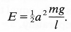 (8.12)
When a damping force is present, however, it is always directed so as to resist the motion, and the work done by it is negative; i.e. mechanical energy is taken from the system by the friction. This energy is converted into heat, and although it is possible to convert heat back into mechanical energy, you can never get as much mechanical energy out as you put heat in (this, roughly speaking, is the second law of thermodynamics). If the damping is very gradual, so that the system almost executes simple harmonic motion, then the total energy will still be given by Equation (8.12), but the amplitude a of the oscillations (the only variable in that equation) will gradually diminish with time, until it becomes undetectable.
When the oscillations are small enough for the restoring force to be directly proportional to the displacement (the situation considered above), then it is usually an equally good approximation to represent the damping force as directly proportional to the rate of displacement, i.e. to the velocity. In the case of a single particle undergoing simple harmonic motion, like the simple pendulum, the additional force to be inserted on the right-hand side of Equation (8.1) may be written -C dy/dt, where C is a constant. This is proportional to the velocity dy/dt, and in the opposite direction to it. The equation of motion of the particle then has three terms, instead of the two in Equation (8.1): the mass times the acceleration is equal to the sum of the restoring force and the damping force. The equation corresponding to (8.1) is therefore
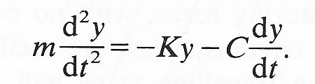
This can be re-written in the following form,
 (8.13)
where 2b = C/m, and w2 = K/m, which corresponds to Equation (8.2) in the case without damping.
Rather than consider the most general motion consistent with Equation (8.13), let us examine once more the case where the particle starts off at the point of equilibrium (y = 0) with a given velocity V; in symbols this condition is
 (8.14)
The complete motion in this case when there is no damping (b = 0) is given by Equations (8.7) and (8.8). The solution of Equation (8.13), and hence the motion of the particle, when there is damping, is of a different form according to whether the parameter b is less than, equal to, or greater than the frequency w. We consider the three cases separately.
(a) b < w.
In this case, the solution is
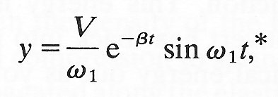 (8.15)
where the quantity w1 is given by
![]()
and is called the reduced frequency or damped natural frequency.* [*The number e is approximately equal to 2.718. The graphs of (a) y = ex, (b) y = e-x, and (c) y = 1 - e-x are plotted in Fig. 8.9. The quantity ex (the 'exponential function') becomes infinitely large, and the quantity e-x tends rapidly to zero, as x becomes infinitely large. Indeed, e-x tends to zero more rapidly than any inverse power of x, such as x-100 or x~1000000. The significance of ex is that it is its own differential coefficient, i.e. d/dx(ex)=ex and d/dx(e-x)=e-x. That is why exponentials occur very frequently in the solution of problems like the present one.]
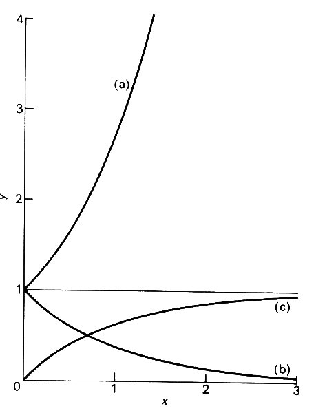
Fig. 8.9. Graphs of (a) y = ex, (b) y = e-x, (c) y = 1 - e-x against x.
The graph of y against t in this case is given in Fig. 8.10 (a),
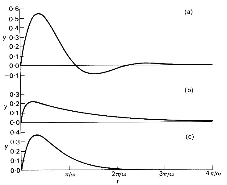
Fig. 8.10. Graphs of y against (when y is given by (a) Equation (8.15), with b = 1/2w, (b) Equation (8.17), with b = 2w, (c) Equation (8.19), with b = w. In each case V/w was taken to be 1 unit of length.
for particular values of b and w. The motion is still oscillatory, with frequency w1 (period T1=2p/w1), but with amplitude a given by
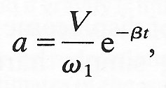 (8.16)
which is reduced by a factor e-bT1 every period (this factor is often called the damping factor). This case is an example of a damped oscillation.* [*The performance of physiological pressure transducers with fluid-filled needles or catheters attached to them is often analysed in this way. Here the diaphragm of the transducer acts as a spring, and overshoots when it is displaced by a pressure signal, the fluid in the catheter providing most of the inertia; thereafter, the overshoot is damped out by the viscosity of the fluid in the catheter. The magnitude and rate of decay of the overshoot is of interest because it obviously determines the fidelity of the transducer in recording pressure changes. For the liquid-filled systems with stiff diaphragms which are usual in circulatory studies a decaying oscillatory response occurs, as in Fig. 8.10 (a). If the damping factor and the damped natural frequency can be determined from calibration manoeuvres, the performance of the system can be predicted over a wide frequency range.]
(b) b > w.
In this case the motion is given by
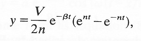 (8.17)
where n = (b2 - w2)1/2 and is less than b.
The graph of y against t is given in Fig. 8.10 (b), for particular values of b and w. In this case there are no oscillations: the pendulum swings out and swings back, coming gently to rest at its starting point again. Strictly speaking, the motions described by Equations (8.15) and (8.17) do not die away until an infinite time has elapsed, since e-bt does not become zero until t = infinity. However, in practice, such motions become undetectable after a finite time; for instance, the amplitude given by Equation (8.16) is reduced by a factor 1/100 by the time bt = 4.6, so a suitable measure of the decay time is
t = 4.6/b (8.18)
The completely damped motion described by Equation (8.17) (called an overdamped oscillation), is the sum of two exponential decay terms. The one which decays more slowly is e-(b-n)t, so the time for decay by a factor 1/100 is 4.6/(b-n). It is interesting to note that if b is very large compared with w, a case of extremely strong damping, then n is approximately equal to b, and b-n is extremely small. In fact, b-n is approximately equal to w2/2b, so the decay time is 8.6b/w2; this is very large compared with 2p/w), the period of the undamped oscillations (w is called the undamped natural frequency). So if you want to damp out unwanted oscillations as quickly as possible, the answer is not to make the damping term b as large as possible; in fact b should exceed w by as little as possible for the fastest decay (without overshoot).
(c) b = w.
This is the critical case which separates (a) and (b), and the motion is given by
y = Vt e-bt (8.19)
Its graph is drawn in Fig. 8.10 (c). This is not much different from Fig. 8.10 (b); this case is significant only because w is the smallest value b can have without oscillations in the motion. The motion is said to be critically damped.
In the same way that simple harmonic motions (and, similarly, standing waves) are damped out in time, so travelling waves, forced by oscillations of a given amplitude and frequency, are attenuated in space. If we travel along with the wave, at the wave-speed c, we observe the wave beside us decaying in time, with a decay time which we may call TD. The amplitude of the wave therefore diminishes with distance from the origin, and a suitable 'decay distance' would be cTD. In many cases of interest (waves on stretched strings, water waves, sound waves), the attenuation is slight and the waves persist for many wavelengths from the origin, so we do not normally need to consider over-damped or critically damped waves (there are exceptions, like surface waves on syrup or pressure waves in the microcirculation: see Chapter 13, §13.4.2). The rate of attenuation of the pressure wave in arteries is quite large, per wavelength, but, as we shall see in Chapter 12, the wavelength is so large compared with the length of the artery that not much attenuation is actually observed.
In the same way that damped simple harmonic motion was seen to differ from simple harmonic motion because of the exponential decay term, so a similar difference can be seen between damped and undamped travelling waves. A damped wave of frequency w, corresponding to the pure sinusoidal wave of Equation (8.10), would be represented by an equation relating the displacement y to x and t, of the following form:
y = ae-kx/l cos {w(t - x/c)} (8.20)
This is of exactly the same form as Equation (8.10), with the propagating oscillations represented by the cos { } term, except that the amplitude of the oscillations decays exponentially as x increases. Here A is the wavelength, and k is a constant which describes the attenuation: the amplitude a e-kx/l is reduced by a factor of 1/100 in a distance of 4.6/k wavelengths. Alternatively, we can say that the wave is attenuated by a factor e-k (the attenuation factor) each wavelength.
Our discussion of travelling waves, damped or not, has been based on the supposition that the medium in which they are being propagated (the stretched string in the example) is infinitely long, so that there is no impediment to the continued propagation of the waves. In fact, of course, no real system is infinite in extent, and we should consider what happens when a travelling wave meets an obstruction. Suppose that the long stretched string of the above example, oscillated at one end, is attached securely at the other end (x = l) so that no displacement is possible there (Fig. 8.11).
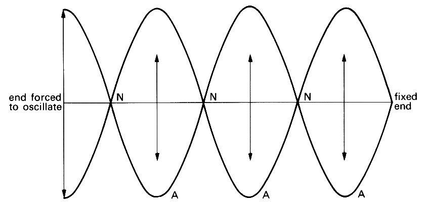
Fig. 8.11. A finite string, of which one end is fixed and the other forced to oscillate with frequency w. The superposition of the incident wave on to the reflected wave forms a standing wave. No displacement occurs at the nodes, N; at the antinodes. A, the amplitude of the oscillation is a maximum.
We ask what becomes of the displacement y, given by Equation (8.10), since that would oscillate between +a and -a at every point, including x = l. It is more convenient if we let the origin of coordinates be at the point x = l, so for simplicity we write x = l + x'; x' is the new coordinate, and is actually negative in the string. Then Equation (8.10) becomes
y = a cos {w(t - x'/c)} (8.21)
and the attachment where y must be zero is at x'=0. The presence of the attachment has the effect of superimposing on to the original wave (called the incident wave) another wave, with the same amplitude and wave-speed, propagating in the opposite direction. This is the reflected wave. The complete equation for the displacement is now
y = a [cos {w(t - x'/c)} - cos {w(t + x'/c)}] (8.22)
At the fixed end (x'=0) and at every half wavelength from it (x' = -pc/w, -2pc/w, -3pc/w, etc.) the displacement is zero at all times; half-way between these nodes are points where the displacement oscillates with double the original amplitude (antinodes; see Fig. 8.11). In fact, the motion is a standing wave; Equation (8.22) can be rewritten as
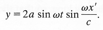 (8.23)
For every value of x', y oscillates in simple harmonic motion, the amplitude of the oscillation being proportional to sin wx'/c, which is of course zero at the nodes and equal to one at the antinodes. The oscillations do not propagate, and clearly represent a standing wave.
The above is an example of total reflection, in which the amplitude, and hence the energy content, of the reflected wave is equal to that of the incident wave. Usually, however, not all the energy of the incident wave is reflected; some of it is either absorbed or transmitted. Suppose that the stretched string is attached, not to a fixed support, but to a support which can move, but whose motion is resisted by some frictional force which dissipates energy (Fig. 8.12).
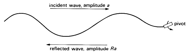
Fig. 8.12. Reflection by a support which can move (e.g. a pivot) but at which energy is dissipated. The amplitude of the reflected wave is smaller than that of the incident wave.
Then some of the energy of the incident wave will be used up in feeding this dissipation, and the reflected wave must have less energy, i.e. a smaller amplitude. This is an example of partial reflection. If, say, the amplitude of the reflected wave of Equation (8.22) were only 80 per cent of that of the incident wave, the displacement would be given by
u = a [cos {w(t - x'/c)} - R cos {w(t + x'/c)}] (8.24)
where R is a constant equal to 0.8. R is sometimes called the reflection coefficient.* [*Here R is the amplitude of the reflected wave, relative to that of the incident wave. More commonly the reflection coefficient is defined as the rate at which energy is transmitted in the reflected wave, relative to that in the incident wave, and that quantity is equal to R2. It is important to know which definition is being used when people refer to the reflection coefficient.] The incident wave is also partially reflected if it encounters some discontinuity in the propagating medium, like a local change in the density or thickness of the string, or a local constraint on its movement, like a bead attached to the string in the middle (Fig. 8.13).
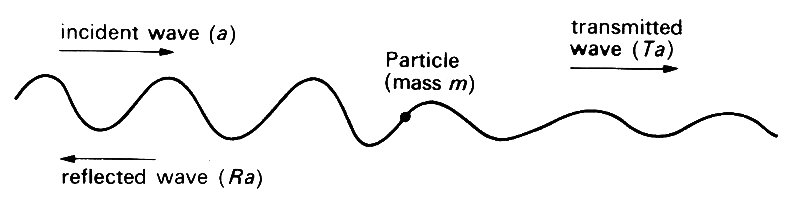
Fig. 8.13. Reflection and transmission of a wave at a discontinuity in the string (here a particle of mass m attached to it, which resists displacement because of its inertia).
In this case a wave continues to be propagated down the string on the other side of the discontinuity but it too has reduced amplitude. This is the transmitted wave; its amplitude would be equal to a times a number T, less than one. T is sometimes called the transmission coefficient; more commonly T2 is so called. If no energy is absorbed, T2 = 1 - R2.
Any discontinuity in a system can be a source of reflections, and if a system contains many such discontinuities, the wave from any point will be a complicated superposition of the incident wave, the reflected and transmitted waves at each discontinuity, the waves generated by subsequent reflection and transmission of the reflected and transmitted waves, etc. The process of reflection, re-reflection etc. does not go on for ever, primarily because of the attenuation of the waves, and also in part because of energy absorption at end-points such as the rough pivot in the above example, or a sloping porous beach in the case of water waves, which absorbs almost all the incident energy.
We saw in §8.2 how a finite stretched string, fixed at each end, can support free oscillations at certain natural frequencies. If a point of the string is oscillated at a given frequency <u not equal to one of the natural frequencies, then waves will propagate from it towards each end, will be reflected there, re-reflected at the other end, etc. The final motion will be a complicated standing wave with frequency equal to the forcing frequency w. If w is equal to one of the natural frequencies, however, the situation is quite different. In that case, the phases of the incident and reflected waves are such that they strongly reinforce each other on each reflection, and the amplitude of the oscillation would continue to grow until the dissipative effects, which would also be growing, become so large as no longer to be negligible. In addition the system would cease to be linear (see below). Energy is continuously being put into oscillations of such a frequency that they can maintain themselves at a constant amplitude in the absence of energy input. The effect of all this extra energy is to increase the amplitude dramatically. The phenomenon is known as resonance. The amplitude of a resonant oscillation is in practice limited by frictional or dissipative effects (or non-linear effects) but unless these are very strong, the ultimate amplitude is still much greater than that of the original forcing. Resonance may be desirable or undesirable. Musical instruments are so designed that of the wide range of frequencies present in the forcing (e.g. the oscillations of a reed) only a few resonate and are thereby amplified into audible sound. In the arterial system, however, resonant oscillations are clearly undesirable, since unusually large pressure oscillations would affect blood flow and might damage the tissues.
The properties of waves, as outlined above, will be applied in Chapter 12 to the wave motions which are present in the mammalian cardiovascular system. All those properties, and some others, will be seen to have widespread relevance. It is important to realize, however, that the relatively simple considerations discussed so far are applicable only when the amplitude of the oscillations is sufficiently small for the restoring force to be proportional to the displacement, and the damping force to be proportional to the rate of displacement. In this case the oscillations, or waves, are said to be linear. The idea of linearity is essentially a mathematical one, but it is of such importance in the theory of wave propagation that it requires some elaboration here.
Suppose that a particular system operates in such a manner that two variable quantities are always related to each other in some way. These might be the velocity and pressure of blood flowing in an artery, measured at a particular station, or the displacement and acceleration of a particle in oscillatory motion, or the mass and oxygen consumption of a living organism; a quite general type of system is envisaged. Let us call the two variables u and p. The relationship between u and p is linear if the graph of u against p is a straight line and u is directly proportional to p; that is:
u = ap (8.25)
where a is a constant. A more general definition of a linear system can be derived from this: if u1 and p1 are one pair of corresponding values for u and p, and if u2 and p2 are another corresponding pair, then the system is linear if (u1 + u2) and (p1 + p2) are also a corresponding pair. A system represented by Equation (8.25) is clearly linear by this definition, whereas a system represented by, say, u = p2, whose graph is a parabola, is not.
Similarly the system represented by Equation (8.2) and the associated conditions at the time of release, which describe simple harmonic motion, is also linear. For instance we saw that the solution
y = a cos wt
corresponds to an initial displacement a (Equation (8.5)), and that the solution
corresponds to an initial velocity V (Equation (8.7)). It is easy to verify that the sum of these solutions, i.e.
corresponds to a state in which the initial displacement is a and the initial velocity V. Again, the reflection of sinusoidal waves described above is a linear process, in that a doubling of the amplitude of the incident wave would result in a doubling of the amplitude of the reflected wave, etc. Furthermore, the system in which the waves are propagated, the stretched string, must be linear in order for the total displacement to be represented simply by the sum of the displacements associated with the incident and reflected waves separately.
The equations governing almost all real physical systems are actually non-linear. For instance, the actual equation describing the oscillations of a simple pendulum is (8.2a) rather than (8.2), and it reduces to (8.2) only if q is small enough for sin q to be approximately equal to q. The error in this approximation is proportional to q3,* [*Because an approximation to sin q that is better than merely q is in fact: sin q = q - q3/6.] which is very much less than q if q is very much less than 1: when q = 0.1, q3 is equal to 0.001. As long as q remains small enough, the real non-linear system, described by Equation (8.2a), will behave almost as if it were linear, and we obtain a good approximation to the behaviour of the real system by analysing the much simpler linear system. The process of converting a small-amplitude non-linear system to a linear one is called linearization. It is a process which is very frequently employed in many fields of application, including the analysis of blood flow in arteries, because linear systems are so much easier to analyse. However, in all practical applications, it is important to verify that the neglected non-linear parts of the equation describing the real system are indeed small compared with the linear ones. If they are not, the non-linearities are important, and their effect must be assessed.
One type of system which can usually be treated as linear, but in which non-linearities become important in certain circumstances, is that of a finite stretched string, forced to oscillate at a frequency close to one of the natural frequencies. A wave is generated at the source of oscillations, and is repeatedly reflected in such a way as to reinforce itself (resonance) so that its amplitude becomes very large. In these circumstances the linear approximation under which the wave was originally analysed ceases to be valid. The detailed, non-linear, analysis of a resonant system is usually very complicated.
The equations of fluid mechanics are non-linear, because of the term representing convective accelerations: Bernoulli's equation (Equation (4.6), §4.7) is an example. This equation relates the pressure p to the velocity u of a fluid in steady motion when viscosity can be neglected. Suppose that fluid is flowing in a horizontal pipe (so that gravity is unimportant) of non-uniform cross-sectional area (so that u varies along it: see §4.6); if the pipe is also elastic, this can be used as a model of blood flow in large arteries, as we shall see in Chapter 12. Suppose too that the flow is oscillatory, and that Bernoulli's equation can be modified to take account of the unsteadiness by a term proportional to the local acceleration du/dt. It would then become
 (8.26)
where k is a constant (with the dimension of length) and r is the fluid density, also supposed constant. In fact the local acceleration term in the real equation describing unsteady flow is more complicated than the one given here, but it is, like this one, linear, so that Equation (8.26) is an adequate model for the present discussion. If the term representing convective accelerations, 1/2u2, were to be neglected. Equation (8.26) would reduce to
 (8.27)
From the above definition, Equation (8.27) is linear while (8.26) is not. Suppose that the fluid velocity were oscillating everywhere with angular frequency w, and were proportional, say, to cos wt. If (8.27) were the governing equation, this could be associated with a pressure oscillation of the same frequency, proportional to sin wt. But if (8.26) were the governing equation, a solution in which u was proportional to cos wt (and hence du/dt to sin wt) would require that u2 be proportional to cos2 wt, which is equal to 1/2 + 1/2 cos 2wt. Thus a velocity wave-form of a single frequency w must be associated with both the mean pressure and a component of frequency 2w, as well as the component of frequency w. This makes the analysis of non-sinusoidal oscillations much more difficult, as we shall see.
A general periodic wave motion is not usually purely sinusoidal. The graph of the displacement of a string against position x at any fixed time, or the graph of blood velocity in an artery against time at a fixed position, may have a very complicated shape (see the last panel of Fig. 8.14). Such a shape can, however, be expressed as the sum of a number of sinusoidal oscillations of different phase and amplitude, and with frequencies which are multiples of the fundamental frequency w (=2p/T), where T is the overall period of the oscillations. The process of splitting up a complicated wave-form into its sinusoidal components is called Fourier analysis. The different frequency components which make up the complete wave are again called the harmonics of the fundamental (cf. §8.2). The number of harmonics required for an accurate representation of the complete oscillation may be large or small. For example, the wave-form shown in Fig. 8.14,
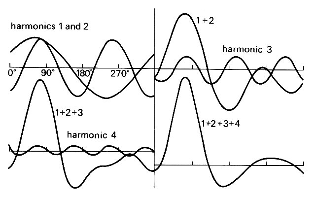
Fig. 8.14. A periodic wave-motion, similar to the graph of blood velocity against time in an artery. Diagrams show how the mean, the fundamental and three harmonics can be superimposed to make up the complete wave-form. The mathematical form of each term is given by Equation (8.28). (From McDonald (1974). Blood flow in arteries, p. 129. Edward Arnold, London.)
which is similar to a velocity wave-form in an artery, can actually be represented by a mean term, a fundamental, and three harmonics. Its equation is
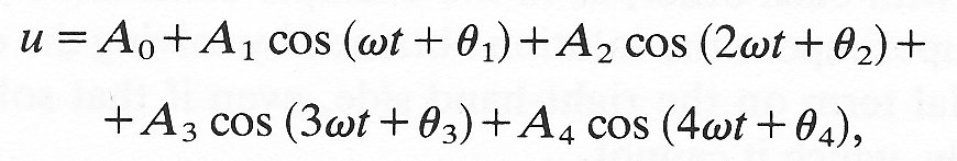 (8.28)
where A0=0, A2/A1=0.97, A3/A1=0.47, A4/A1=0.14, q1=-58°= -1.01 rad, q2=-151° =-2.64 rad, q3=+124°=2.16 rad, q4=+86°=1.5 rad. The way the three components add up to form the complete wave is illustrated in Fig. 8.14.
Fourier analysis can be applied to a wave-form of any shape. It is a process which considerably simplifies the analysis of oscillations and waves in linear systems, but is of little value in non-linear systems. Suppose that we wish to calculate the blood pressure p in an artery from a measured oscillatory velocity u, by the use of Equation (8.27). We can express the velocity as the sum of sinusoidal wave components, as in Equation (8.28). We can also use Equation (8.27) to calculate the pressure oscillation corresponding to a single component of the velocity oscillation; i.e., corresponding to
u = An cos (nwt + qn)
the equation, with a zero on the right-hand side, gives
p = rknAn sin (nwt + qn)
(The constant term on the right-hand side of Equation (8.27) is equal to a mean value of the left-hand side, i.e. p0/p.) We can finally add up all the sinusoidal pressure modes, derived in this way, to obtain the composite pressure waveform, and this addition is permitted since the system is linear. In the non-linear system represented by Equation (8.26), however, all the frequency components interact with each other, as in the example considered above. It is not permitted to superimpose the solution obtained by solving the equation with a single sinusoidal term on the right-hand side, even if that solution could be obtained simply, which it cannot.
The pressure waves which exist in large arteries are approximately linear, as we shall see in Chapter 12, and their principal features can be derived from linear theory. There are some features, however, which can be explained only with the aid of non-linear ideas. These include the steepening of the pressure waves in some circumstances as they propagate down the arterial tree, and the large amplitude oscillations which may be heard in arteries which are constricted by a high pressure cuff (the co-called Korotkoff sounds, see §14.4.3). Non-linear behaviour is also seen in veins (see Chapter 14).