We turn now to an examination of the patterns of blood flow within arteries, with the twofold aim of interpreting measurements of blood velocity and understanding the influence of local blood flow on physiological processes in the artery wall. We shall first consider experimental information about flow patterns within large arteries, and then go on to discuss physical mechanisms which lead to these patterns.
12.8.1 Velocity profiles in large arteries. In the last few years, a number of techniques have been developed for the measurement of blood velocity in arteries in the living animal. Some of these (in particular the electromagnetic method, utilizing cuff or catheter-tip probes) are sensitive to the flow in all, or a considerable part, of the lumen of the vessel, and thus measure a spatially averaged velocity. Others, notably the hot-film and pulsed Doppler techniques, can be used to plot blood velocity from point to point within a vessel. The ultrasonic Doppler technique has tremendous promise, since it can produce an almost instantaneous plot of the velocity distribution across a vessel, without the necessity of inserting a probe into it (and potentially even in the intact animal); but it is still in the process of development, and has so far yielded only a little information about arterial flows; we shall therefore concentrate on the studies with hot-film probes.
The technique of hot-film anemometry employs tiny, velocity-sensitive probes mounted near the tips of hypodermic needles or catheters, which are inserted into the artery. Such probes are sensitive only to flow within a millimetre or less of their surface; thus they can be used to plot blood velocity from point to point within a vessel. In addition, since they are capable of registering velocity fluctuations up to frequencies in excess of 500 Hz, they can be used to study disturbed and turbulent flows in blood vessels.
The technique has revealed a good deal about the velocity distribution in the aorta of the dog, and a few observations have been made in man; but even with the smallest probes, it has not been possible to explore the boundary layer itself in either of these species. This is because the boundary layer is very thin. Even the smallest hot-film probes become unreliable near the artery wall, partly because the signal is influenced by the proximity of the wall, and partly because the vessel wall is moving radially. This means that the relative position of the (fixed) probe and the wall changes during the cardiac cycle, and that appreciable radial velocities occur in the blood which distort the recording of the longitudinal velocity. This unreliability of hot-film probes very near vessel walls means that they can only be used to study the velocity profiles in large arteries, and in the dog this means the aorta. Even there, only certain sites are accessible, because of problems in surgical exposure, and because care must be taken to avoid distorting the vessel during measurement; it has been found repeatedly that the velocity profile changes dramatically if the vessel is distorted. A final problem encountered in reporting and interpreting these studies is that different workers have not always precisely defined the sites and the planes at which they have traversed vessels. As will be seen, local geometry has important effects on the flow, and many inconsistencies between different studies or different animals are probably attributable to this. In what follows, we concentrate on the features which have been consistently observed.
If we examine the mean velocity profile (i.e. the velocity profile constructed from time-mean measurements) at some of the sites which have been studied in the dog (Fig. 12.38),
Fig. 12.38. Velocity profiles in the aorta of the dog. For each graph, the mean velocity at each site on the vessel diameter is expressed relative to the centre-line mean velocity. (From Schultz (1972). 'Pressure and flow in large arteries'. Cardiovascular fluid dynamics (ed. Bergel), vol. I. Academic Press, New York.)
we can see that it remains blunt throughout the length of the aorta, with only the measurements closest to the wall showing retardation of the flow compared to that in the centre of the vessel. Close to the heart, virtually no retardation is detectable anywhere; the blood moves as a coherent 'slug' and the boundary-layer is confined to a wall-region too narrow to be observed; in practice, this means that it is less than 2 mm thick.
This is true throughout the flow cycle in the thoracic aorta. In Fig. 12.39,
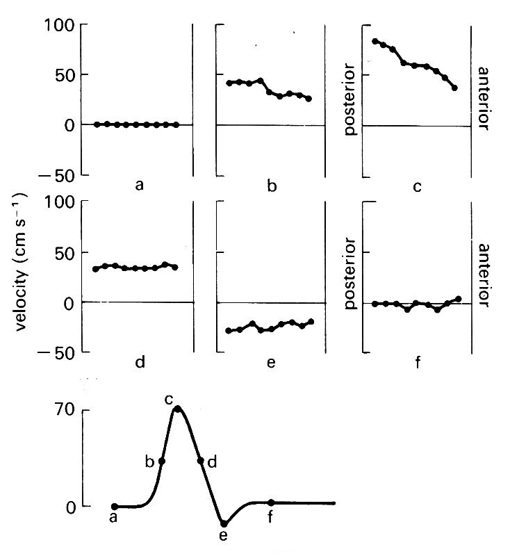
Fig. 12.39. Instantaneous velocity profiles at six different times during the cardiac cycle in the ascending aorta of the dog. The lower figure shows schematically the velocity wave-form, with the six times marked on it.
instantaneous velocity profiles in the ascending aorta are shown at six times during the cardiac cycle. It can be seen that a marked skew occurs during forward flow; but there is no evidence at any stage of velocities being preferentially lower close to the wall. Some workers have approached the problem of studying these very thin boundary layers by using the pig and the horse, which have larger aortas than the dog. In the pig, radial wall movement was eliminated by splinting the vessel with a rigid external cuff; but even in these circumstances it was not possible to examine the boundary layer in any detail, because it was less than 1.5 mm thick. On theoretical grounds it is expected to be thin, as we shall see later.
These studies have, however, revealed considerable detail about the behaviour of the flow in the core of the vessel. At the entrance of the aorta, a centimetre or two downstream from the aortic valve, the velocity profile is usually symmetric during systole, at least in the plane of the main curvature of the aortic arch (this is the only one accessible to study, and is virtually antero-posterior at that level - Fig. 12.40, lower site).
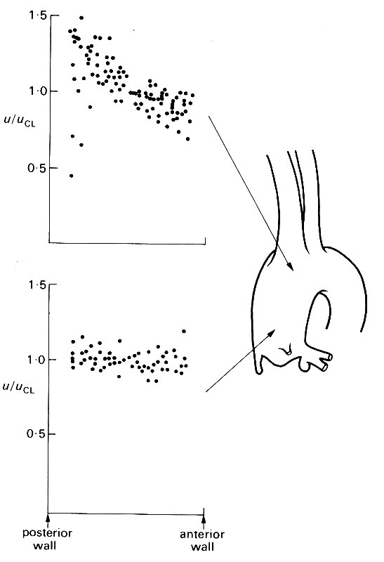
Fig. 12.40. Velocity profiles at peak systolic velocity across two diameters in the ascending aorta of the dog. All velocities (u) are expressed as a ratio of the centre-line velocity (uci), and all radial positions as a ratio of the vessel radius. The profiles at both sites are from several dogs; in every case they were measured in the plane of the main curvature of the aortic arch.
This is the form which is to be expected for an entrance flow (see §5.2), but there are several less familiar features.
First, velocity wave-forms at this site frequently show low-frequency disturbances during systole, which may be quite variable from beat to beat, or may be so reproducible that they skew the velocity profile on each beat, usually in late systole. Such disturbances may be residues of the eddying known to occur within the ventricle (§11.5.2), or may arise during passage of the blood through the aortic valve. In studies with catheter tip probes where records of velocity have been made within the ventricle, disturbances have been seen during systole as well as diastole. This suggests that the disturbances set up in the ventricle during diastole do persist into the ejection phase, and may therefore be the source of the aortic flow disturbances. However, this sort of evidence is not conclusive because catheters in the ventricle may be jerked about during systole, causing distortion of the velocity signal, and to date the source of these low-frequency flow disturbances in the ascending aorta has not been firmly established.
A second interesting feature of the flow is that this symmetry of the systolic velocity profile is lost as the flow travels up the ascending aorta and into the arch; the flow close to the inner (posterior) wall of the arch is accelerated, producing a marked skew (Fig. 12.40 upper profiles).
The skewing of the flow as it enters the aortic arch is a constant finding. A number of explanations have been put forward; for example, the velocity profile may be influenced by the proximity of the major branches coming off the aortic arch, which are expected to cause considerable local distortion of the flow (see, for example, Fig. 12.47). Another explanation is related to the tight curvature of the aortic arch. In flow through such a bend, a transverse pressure gradient is set up, so that along a diameter in the plane of the curve (i.e. aligned like the spoke of a wheel) the pressure will rise towards the outer wall. In an inviscid flow (such as that in the core of the aorta) this causes relative retardation of the streamlines near the outer wall; the effect is explained in detail in Chapter 5 (§5.8). This explanation would also fit the observed fact that the skew disappears as the velocity falls, and recurs during flow-reversal in early diastole. It would also explain why the magnitude of the skew varies from animal to animal, since this depends on the local geometry (radius of curvature of the bend, and diameter of the vessel). This of course would also be true if the skew was due to vessel branching, and it is quite likely that both mechanisms play a role.
Profiles have also been examined at right angles to the plane of the aortic arch. This plane is not accessible close to the aortic valve, because the pulmonary artery overlies the aorta, but can be examined more distally, at the entrance to the arch (roughly level with the upper site in Fig. 12.40). Here again, skewing occurs, with higher velocities towards the left wall during systole. This is unlikely to be a curvature effect, because the vessel is relatively straight in this plane, and we have as yet no clear explanation for it.
During diastole, the cross-sectional average velocity, as measured, for example, by a cuff electromagnetic flowmeter, is very close to zero in the ascending aorta. However, hot-film measurements show that the blood does not actually come to rest during diastole. Local backflows, affecting only part of the cross-section of the vessel, and compatible with drainage into the coronary arteries, can be observed. Also, at the entrance to the aortic arch flow may simultaneously be moving forwards on one side of the vessel and backwards on the other. This suggests a circulating flow, presumably associated with drainage into the arch branches, where forward flow can be maintained during diastole.
Measurements in the proximal descending aorta can only be made in a plane orthogonal to the main curvature of the arch. Here too, circulating flow may occur during diastole, but in systole there is strikingly little evidence of any influence from the major branches just upstream. The systolic profiles remain blunt, with a slight skew towards the right wall; the mean profiles are usually symmetrical (Fig. 12.38). More distally, the first hint of 'rounding' of the mean profiles, implying viscous influences and the growth of the boundary layer, can be seen.
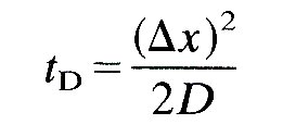
In the abdominal aorta and the major branches, hot-film probes are usually too big for detailed studies in the dog. Recently, however, measurements have been made in the horse, where access is possible much more peripherally (in a large horse, the aorta may have a diameter of 5 cm at its origin, and major branches like the brachiocephalic or iliac arteries are 1.3 cm across). At first sight, this might seem an obvious solution to the problem of examining the boundary-layers also; but in fact the boundary-layer thickness in unsteady flow is independent of vessel diameter, and is proportional to (n/w)1/2 (see §12.3.3). The kinematic viscosity of blood at high rates of shear is much the same in the majority of mammals, so that boundary-layer thickness depends on l/w1/2, and thus varies inversely with the square root of heart rate. Between different species, therefore, the thickness of the boundary-layer will only increase if the heart rate is lower.
In fact, heart rate does tend to fall with increasing body size, and therefore there are good reasons for studying larger animals. The horse, for example, has a heart rate of 30-50 min-1, compared to 80-120 min-1 in the dog; thus the boundary-layer is expected to be 60 per cent thicker in the horse, and has proved to be accessible to study, though not yet in detail. In Fig. 12.41,
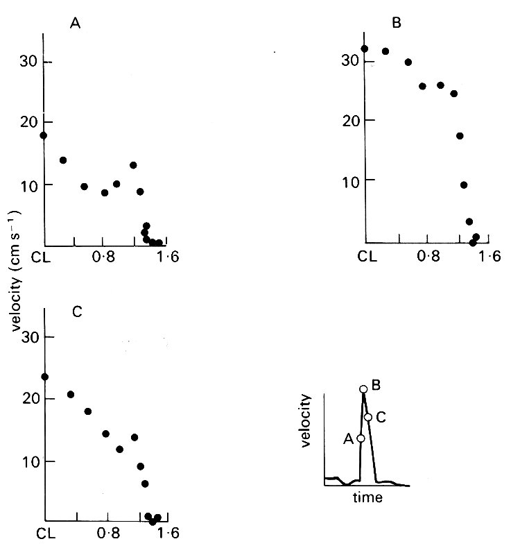
Fig. 12.41. Half-width velocity profiles (from centre-line to right wall) in the descending thoracic aorta (10 cm distal to the arch) of the horse. The inset velocity wave form shows the points in the cycle at which the profiles were constructed. Ordinate: velocity of blood (cm s-1). Abscissa: distance from centre-line (CL) (cm). Vessel diameter 2.69 cm. a = 19.4; peak Re = 2536. (After Nerem, Rumberger Jr, Gross, Hamlin, and Geiger (1974). 'Hot-film anemometer velocity measurement of arterial blood flow in horses.' Circulation Res. 34, 193-203.)
velocity profiles in the descending thoracic aorta are shown at three instants during systole. They confirm that the boundary-layer is thin (3.4 mm) during forward flow; but it must be remembered, in examining the boundary-layer itself, that measurements extremely close to the wall may not be very accurate because of wall-movement and radial flow. High frequency velocity fluctuations, indicating significant flow disturbance or turbulence, were frequently encountered in the thoracic aorta, but not further downstream.
In the abdominal aorta, several influences affect the velocity distribution. Immediately below the point where the mesenteric, coeliac, and renal arteries branch off the aorta (the anatomy in this region is similar to that in the dog. Fig. 12.1), velocities fall markedly, reflecting the large diversion of blood into these branches. The velocity profile becomes more rounded, suggesting the influence of viscous forces, and also skewed, presumably in relation to local upstream drainage into a branch. The peak Reynolds numbers in this region lie between 200 and 800, and flow disturbances were not seen. Further downstream, very close to the termination of the aorta, the most striking feature was that the highest velocities were observed off the centre-line of the vessel, so that the systolic profile was M-shaped. It is not clear how such a pattern could be set up during forward flow as a result of the proximity of the branching. It seems likely to be an oscillatory flow phenomenon, as can be seen occurring in a straight, unbranched pipe in Fig. 5.9, §5.6.
A few measurements have also been made in the iliac arteries, distal to the termination of the aorta. There, the profiles during systole are relatively symmetrical and markedly rounded. More distally than this, measurements have not been made with hot-film probes in any species.
12.8.2 Physical mechanisms underlying the velocity profiles. Oscillatory flow in a long, straight, rigid tube when an oscillatory pressure difference is applied between the ends has been described both in Chapter 5 and in §12.3 of this chapter. Experimental observations on such a flow, which show very close agreement with theoretical predictions, are shown in Fig. 12.42.
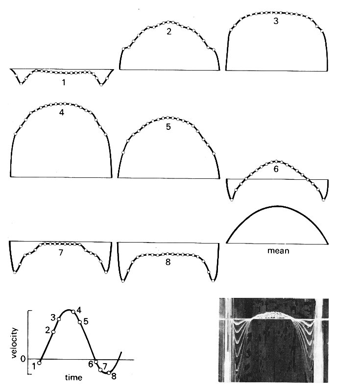
Fig. 12.42. Instantaneous velocity profiles at eight different times during a cycle of oscillating flow in a long, straight rigid pipe. The times are marked on the flow-rate wave-form which is shown at bottom left and which consists of a sinusoidal oscillation super-imposed on a steady flow, so that there is only a short period of backflow. The measurements were made far from the entrance of the pipe, so that the mean flow had a fully developed, Poiseuille profile (also shown). The flow conditions were chosen to be appropriate to those in the aorta: mean Reynolds number Re = 1785, Womersley parameter a. = 20.5, peak velocity 2.74 times mean velocity. The measurements were made by 'marking' the flow with lines of tiny hydrogen bubbles, generated by pulsing electrical current through a fine wire stretched across the flow. These bubbles are carried with the flow, and are photographed after a known time interval (inset); the velocity at each point on the diameter during this interval can then be calculated. (Data reproduced by courtesy of Mr. P. Minton and Dr. M. Clamen.)
These observations are not entirely applicable to flow in the aorta because, as will become clear below, the steady component of the aortic flow is not fully developed. The oscillatory components, on the other hand, probably are appropriate.
In this section, we consider steady and unsteady flow near the entrance of a vessel, the effect of vessel curvature, and the flow pattern near sites of branching. We shall neglect the distensibility of the artery wall, for although that is of central importance in determining the local pressure gradient as the pulse-wave propagates, it does not affect the flow-rates and velocity profiles driven by the pressure gradient. The reason is that the wavelength of the wave is very much longer than the distance travelled during any one pulse by an individual fluid element, because the wave-speed is much greater than the blood velocity (see §12.3.5). For instance, the wavelength of the pulse in the dog's aorta is 3-4 m, while the distance travelled by a representative fluid element, which is equal to the mean velocity multiplied by the pulse period, is 10-20 cm. This means that the segment of artery traversed by a fluid element during one heart-beat is approximately uniform in cross-sectional area; the fact that it varies over a distance of one wavelength is irrelevant, particularly since that variation is only about 10 per cent. Elasticity would be important only in circumstances in which passage of the wave caused significant variation of cross-sectional area within a length-scale of about 10 cm; this may happen when the wave-front becomes very steep (see §12.5), but does not normally occur.
The entrance region. The entrance length for steady flow in a straight tube can be calculated by assessing where the boundary-layer comes to occupy the whole radius of the tube (Equation (5.4)). In unsteady flow the mean profile grows with distance from the entrance as it does in steady flow, though it has superimposed upon it everywhere the time-varying oscillatory profile, whose form is dominated by the local value of a. The observer making measurements of the velocity profile at any instant in the cycle will see a velocity profile which is a combination of the steady and unsteady components (as in Fig. 12.42). We can calculate the entrance length for the oscillatory component of the flow by assessing where the thickness of the boundary-layer growing from the entrance (d1) becomes equal to the thickness it would have in fully developed oscillatory flow (d2). The boundary-layer thickness in steady flow was defined (§5.3) as the distance from the wall at which the fluid velocity reaches 99 per cent of its value outside the layer. This distance is equal to 3.5 (nx/u)1/2, where n is the kinematic viscosity of the fluid and u is the core velocity; x is the distance from the entrance (see Fig. 5.5, §5.2). The same formula holds at any time for d1, if u is the instantaneous core velocity. The oscillatory boundary-layer thickness, d2, similarly defined, is equal to 6.5 (n/w)1/2 for an oscillation of angular frequency w. This leads to the following equation for the unsteady entrance length l1:
l1 = 3.4 u/w (12.28)
In the aorta of a dog, for example, the heart rate is about 2 Hz (so w = 4p) and the amplitude of the largest unsteady velocity component is about 40 cm s-1, so that the largest possible instantaneous value of l1 is about 10 cm. For most of the cycle, because the instantaneous value of u is small, and for the components of higher frequency, the unsteady entrance length will be considerably smaller (and will be zero during flow reversal).
The mean flow will continue to develop beyond this point. This development is not affected by the oscillatory components, because, far from the entrance, the oscillatory boundary-layer is much thinner than the developing mean boundary-layer, and thus only influences a narrow region very close to the wall where the mean velocity is in any case very small. We can therefore use the simple relationship of Equation (5.4) (l = 0.03 d Re, where d is the tube diameter and Re is mean Reynolds number) to estimate the entrance length for the mean flow. In a dog's aorta, for example, with diameter 1.5 cm and mean velocity 20 cm s-l, the mean Reynolds number is approximately 800, and the corresponding entrance length is approximately 36 cm, which is almost the whole length of the aorta. In a human aorta, with d = 2.5 cm, u = 20 cm s-1, the entrance length is approximately 94 cm, which is greater than the length of the aorta. In these calculations we have neglected all effects of bends and branches, so that the estimated lengths are only approximate. However, the main conclusion remains, that as far as the mean flow is concerned almost the whole aorta is an entrance region. If we consider small arteries on the other hand, both d and the mean Reynolds number are smaller and the entrance length occupies a much smaller proportion of the vessel; e.g. in a dog's femoral artery, with d = 0.4 cm, u = 10 cm s-1 (Table I), the value of / is approximately 1.2 cm, a small fraction of the total length.
We have seen that the velocity profiles in the core of the aorta will be more or less flat, and the boundary-layers thin. Factors which might modify these predictions are the curvature of arteries, especially at the arch of the aorta, and the presence of branches. We now examine these effects.
Curvature of the aorta. The steady motion of fluid in a curved tube was described in Chapter 5 (§5.8). Far from the entrance, the faster moving fluid in the centre of the tube is swept to the outside wall of the bend, because its inertia makes it respond less readily to the transverse pressure gradient which is forcing it round the bend. It is replaced by the slower moving fluid near the walls, which moves round the walls towards the inside of the bend. In this way secondary motions are set up, and the axial velocity profile is distorted in the manner shown in Fig. 5.16 (§5.8), with higher velocities near the outside wall.
Near the entrance of the tube, on the other hand, the initially flat velocity profile is skewed so that higher velocities occur near the inside wall (Fig. 5.17, §5.8); this occurs in the aorta (Fig. 12.40). There are thin boundary-layers on the walls near the entrance, as usual, but because of the higher core velocity towards the inner wall, the boundary-layer is thinner there, and hence the velocity gradients (and thus the wall shear-rate) are greater. However, the higher pressures which occur at the outside of the tube (Fig. 12.43)
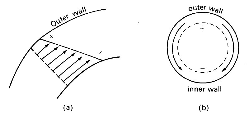
Fig. 12.43. (a) Velocity profile in a curved tube near the entrance (ignoring the boundary layer). + means high pressure, - means low pressure. (b) The pressure difference from + to - drives secondary motions in the boundary layers, as indicated by the arrows.
to force the rapidly moving core fluid round the bend, also act on the slower moving fluid in the boundary-layer. This is therefore forced round the walls towards the inside (as in fully developed flow) so that the boundary-layer thickness on the inside increases relative to that on the outside, and the shear-rate decreases on the inside. Hence the initial distribution of shear-rate is reversed; this is predicted to happen after about one diameter. Such a flow pattern is not discernible in experiments to measure velocity profiles in the aorta, as described above (Fig. 12.40), because the boundary-layer is undetectable. However, the effect on wall shear-rate should be seen in experiments to investigate the transport of substances across vessel walls, when the rate of transport depends on wall shear-rate or shear-stress (see §12.9.2.).
This description strictly applies only to steady flow. In oscillatory flow, regardless of the value of a, it will apply very near the entrance. Further downstream when a is large it will apply only to the mean flow; for smaller values of a (less than about 1), it is expected to apply everywhere. This means that our predictions of the velocity profiles in the proximal aorta are largely unchanged by the presence of oscillations, but the flow further downstream will be a complicated superposition of a mean flow, with higher velocities near the outside, and oscillatory components, with higher velocities near the inside.
Branched vessels. In the analysis of wave reflection at arterial junctions the local flow pattern is unimportant. This means that the detailed geometry of the junction can be ignored, and represented solely by the cross-sectional areas of the arms of the junction. Much more geometrical detail is required, however, for a prediction of the detailed flow patterns. We need to know the angle at which a branch initially comes off its parent vessel, and the angle which it ultimately makes with it (the two are usually different; see Fig. 12.2); we need to know the curvature of all the walls at a junction, including the sharpness of the flow divider; we need to know the way in which the area and shape of the parent tube change as the junction is approached. At present, however, very little of this information is available. It can only be obtained by painstaking measurements of casts of arteries, carefully made at physiological values of transmural pressure and length.
Even if we knew all the geometrical details, prediction of the flow patterns would be very difficult, because there have been very few experimental or theoretical studies of flow in branched tubes, steady or unsteady. We can therefore only make very general predictions about flow in arterial branches.
The type of junction about which most is known is a symmetric bifurcation with equal flow-rates out of each daughter tube (Fig. 12.44),
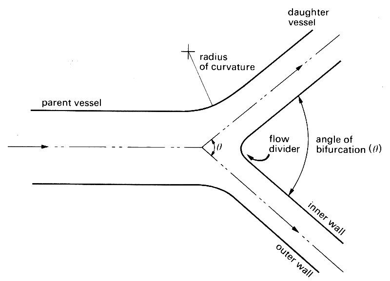
Fig. 12.44. Diagram of a symmetrical bifurcation, illustrating the notation used in the text. Flow direction marked by arrows.
for which a number of experiments have been done with air or water flowing steadily in glass or perspex models. Even with this arrangement, the flow depends on several different quantities. These include the area ratio of the junction (summed area of daughter tubes divided by area of parent), the angle of branching, the radius of curvature of the outside walls of the junction and of the flow divider, the Reynolds number of the flow entering the junction from the parent tube, and the velocity profile in the parent tube. Model experiments have been performed on junctions (representative of the airways of the lung) with area ratios of 1.2, branching angles of 70°, and Reynolds numbers between 100 and 1000. In large blood vessels there are very few symmetric bifurcations, the only familiar one being the human aortic bifurcation, which normally has an area ratio of 0.8 and a branching angle of about 70°. Nevertheless the mean Reynolds number there is about 400, and the results of the model experiments will give an idea of the principal features of the flow.
The most obvious feature is that the flow is split into two. Thus if we suppose the upstream velocity profile to be approximately symmetrical, we see that immediately after the flow has passed the flow divider the greatest velocities will be very close to the inside wall, next to the flow divider itself. The velocity of the fluid in contact with that wall must be zero, so a new boundary layer develops from the flow divider, where the shear-rate is very high. The axial velocity profile in the plane of the junction is expected to resemble that shown in Fig. 12.45 (a).
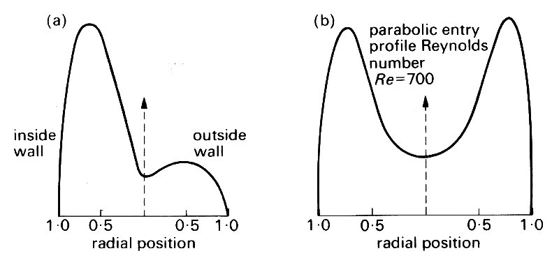
Fig. 12.45. Measured velocity profile 2 diameters downstream of a symmetric bifurcation, at a parent tube Reynolds number of 700 (Poiseuille flow in the parent tube), (a) Profile in the plane of the junction; (b) profile in the perpendicular plane. (After Schroter and Sudlow (1969). Resp. Physiol. 7, 341-55.)
Another obvious feature of the flow is that each of the two streams is made to turn a bend. This means that, as in a uniform curved pipe, secondary motions are set up, as shown in Fig. 12.46, and these maintain the highest velocities near the outer wall of the bend, i.e. the inner wall of the junction (Fig. 12.44). Furthermore, the secondary motions are sufficiently strong to sweep some of the faster moving fluid round to the top and bottom walls, with the result that the velocity profile in the plane perpendicular to the junction has an M-shape, as shown in Fig. 12.45 (b). The secondary motions were visualized by introducing smoke into the flow (Fig. 12.46).

Fig. 12.46. End view of the daughter tube of a symmetric bifurcation (with Poiseuille flow in the parent tube), showing the secondary motions. The flowing fluid was air, and the flow patterns were revealed by smoke injected into the outside wall of the daughter tube. (From Schroter and Sudlow (1969). Resp. Physiol. 7, 341.)
The flow patterns change with distance downstream until, at a distance comparable with the usual entrance length (Equation (5.4)), Poiseuille flow is again set up in each branch. However, the initial development of the flow is considerably different from simple axisymmetric entry flow, because the secondary motions help to maintain the peak velocities near the inside wall for a distance of several diameters.
The velocity profiles of Fig. 12.45 show that the shear-rate at the wall remains high on the inside walls of the junction, not only at the flow divider, but for some distance downstream and for some distance round the circumference of the daughter tubes. On the outside wall of the junction, however, the shear-rate is very low. Indeed in many of the experiments, regions of reversed flow are reported on the outside wall just downstream of the bifurcation, indicating flow separation (see Chapter 5, §5.7>/a>). Whether or not the flow through a symmetric bifurcation separates depends on whether there is an adverse pressure gradient at the wall, tending to slow down the flow. In the model experiments, there was an adverse pressure gradient, because of both the expansion in area (not usually present in the aorta), and the sharply curved walls at the outside of the junction. It did not occur in more smoothly curved models.
The curvature of the walls at the aortic bifurcation is not normally very sharp, so the flow is believed to remain attached. However, if the geometry were distorted by disease, separation might occur, and this would be associated with local reversal of flow direction, and reduced wall shear-rates. This would increase the likelihood of turbulence developing there, and could influence mass transport across the artery wall; both of these topics are dealt with later in this chapter.
The only type of asymmetric junction in which the flow has received attention is that in which a daughter tube branches at right angles off an otherwise uniform parent (Fig. 12.47).
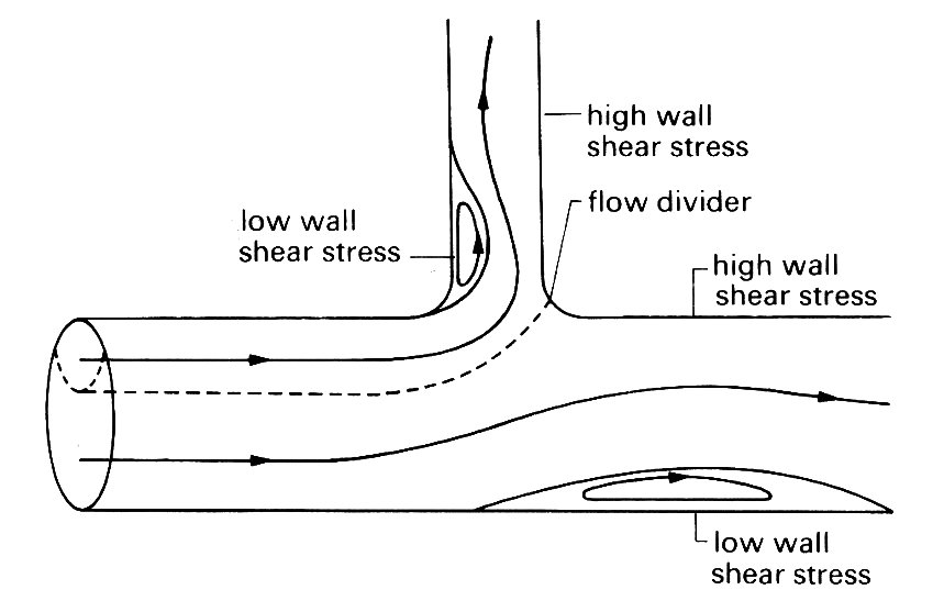
Fig. 12.47. Longitudinal section of an asymmetric junction. Dashed line: surface dividing the fluid which flows down the side branch from that continuing in the main tube; solid lines: streamlines; note also the closed eddies in regions of separated flow.
This is not a good model, even for those cardiovascular junctions in which the ultimate angle between the parent vessel and the branch is a right angle (e.g. where the intercostal or renal arteries come off the aorta); thus the flow pattern in such a junction is an oversimplification of the real flow, but it has a limited value because the geometry is precisely known, and the junction is asymmetric.
Experiments with dye in steadily flowing water have shown that the surface dividing the fluid which flows down the branch and that which continues in the main tube is clearly delineated (Fig. 12.47). The furthest downstream point of this surface lies somewhere on the part of the junction wall opposite to the oncoming flow, which is analogous to the flow divider in the previous example. The exact location of this point depends on the relative flow-rates in the two tubes. It is a stagnation point, where the fluid velocity even just outside the boundary-layer is zero, but the boundary-layer is very thin there, and a little way downstream from it in either direction is a region where the wall shear stress is very high. The flow is generally observed to separate from the inner wall of the junction, and a region of reversed flow and low shear occurs on this wall just downstream of the junction. Strong secondary motions are set up in the branch. Sometimes, separation occurs also in the main tube, at a point roughly opposite the entrance to the side branch. This is because the sucking of fluid down the branch creates a low pressure zone in the parent tube, just downstream of which an adverse pressure gradient occurs. Typical paths taken by particles in the plane of symmetry are also shown in Fig. 12.47.
Recently, quantitative experiments have been performed in a cast of a dog's aorta, in which the shear stress at various sites on the wall was measured. The measurements confirm the above qualitative description of the flow pattern, although because the branch comes off initially at a small angle and then curves rapidly the separated region in the daughter tube may be displaced downstream or may be absent altogether. The results also show clearly that very small perturbations to the geometry of the vessel wall at a junction can have a profound effect on the local flow. In one artery, the flow divider tip (see Fig. 12.47) protruded very slightly into the lumen of the tube (by less than 1 mm), but still that was enough to create another small region of separated flow on the wall of the main tube just beyond the flow divider.
It is clear that the patterns of flow in branching arteries are very complicated, involving secondary motions, and contiguous regions of high wall shear (where the boundary-layer is thin) and of low wall shear (where flow separation may occur). The complicated distribution of wall shear stress may have important implications for the distribution of early atheroma, if that is in any way associated with wall shear (§12.9.2).
12.8.3 Stability and turbulence. In very viscous, or slowly moving fluids (i.e. at low Reynolds numbers), the motion is orderly, with well-defined streamlines and the transfer of material, momentum, and energy across the streamlines taking place only by molecular motion (i.e. diffusion). Such flow is termed laminar: Poiseuille flow is an example. However, it must be made clear that laminar flow may be steady or unsteady, and may have a very complicated structure because of the presence of vortices or secondary motions. A characteristic of laminar flow is that disturbances within it die out due to viscous action. The hallmark of turbulent flow is that it contains disturbances which are random in amplitude, frequency and direction and do not die out (Chapter 5).
As the Reynolds number of a laminar flow is increased, the damping of small disturbances is decreased; ultimately, a critical Reynolds number is reached, beyond which the flow is no longer stable and at least some disturbances are amplified. When Re in a flow exceeds this value, and sufficient time is available, this amplification leads to turbulence. The critical Reynolds number for fully developed pipe flow, based on average velocity and pipe diameter, is usually given as approximately 2300, although it may be considerably higher if great care is taken to avoid introducing disturbances into the flow. However, if an already turbulent flow is slowed down so that Re falls, the turbulence will always persist until Re is below about 2300. The disturbances that initiate turbulence may come from a number of sources and their magnitude has a considerable influence on the critical Reynolds number. The usual sources are eddying upstream (e.g. in the reservoir) or roughness of the pipe wall.
Because the eddies which represent turbulence in a flow are random in size and velocity, they will therefore be 'seen' (for example, by a velocity sensor at a point in the flow) as fluctuating velocity components superimposed upon the bulk flow velocity. An example of turbulent pipe flow is shown in Fig. 12.48.
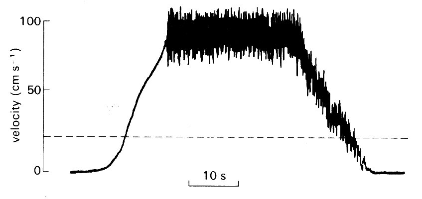
Fig. 12.48. Turbulent flow. Record made with a hot-film probe in a pipe in which the flow-rate was slowly increased until turbulence occurred, and later stopped. Peak Reynolds number 9500. The dotted line shows the velocity corresponding to the usual critical Reynolds number of 2300. (After Nerem and Seed (1972) 'A'; in vivo study of aortic flow disturbances'. Cardiovasc. Res. 6, 1-14.)
Strictly speaking, a flow can only be characterized as turbulent if such fluctuations can be demonstrated to be present in all three dimensions, but in practice the process has been so well characterized in many fluid dynamic situations that fluctuations in one dimension which have the appropriate characteristics are sufficient identification. Apart from illustrating the high frequency velocity fluctuations. Fig. 12.48 illustrates a number of other points about the onset and decay of turbulence. First, turbulence does not appear until Reynolds numbers greatly in excess of the usual critical value of 2300 have been reached. This may in part be because accelerating flow is more stable than steady flow, and in part because the flow upstream was free of disturbances due to the design of the apparatus. Secondly, the turbulence persists as the flow is decelerated, even at Re below 2300. This is partly because decelerating flow is inherently less stable than steady flow, and partly because existing eddies take a finite time to decay.
Since the turbulent eddies cover a wide range of sizes, and are carried with the flow, the velocity seen by a stationary probe will contain fluctuating components having a wide range of frequencies, and a frequency distribution will exist. This can be characterized in a number of ways (for example, by Fourier analysis, §12.2.5) and expressed as a graph of velocity (or energy) against frequency. Typically, this spectrum is centred on some frequency f0, and velocities diminish as frequency becomes both very large and very small compared with this value f0. The value of f0, the 'centre frequency', is dictated by the size of the largest eddies, and these depend on the geometry of the flow. In a pipe flow, for example, the largest eddies have a diameter comparable to that of the pipe, d. Thus if the flow velocity is u, the value of f0 is approximately equal to u/d. The precise point in the spectrum where the maximum amplitude of velocity or energy comes is dictated by a number of interacting and often complicated features of the flow, including local and upstream geometry, and fluid viscosity.
It is unfortunate from the point of view of arterial flows that most of the engineering studies of transition and turbulence have been carried out when the underlying mean flow is steady, and there have been few studies of the stability of unsteady pipe flows. Those which have been carried out have involved flows in which the oscillatory components were small compared to the mean, so that the mean flow properties dominate the flow; this is unlike the situation in large arteries, where the peak velocity may be four or five times greater than the mean.
Until recently, therefore, discussion about the onset of turbulence in arteries has been largely speculative, and based on comparison with steady flow regimes. Such speculation has suggested that turbulence might occur during systole in the larger arteries, and the few attempts made to examine arterial flow in the living animal, by direct cinematography of injected dye, or by cineradiography, have tended to bear this out. Such flow visualization techniques are, however, difficult to interpret in unsteady flow, since they are observed for short periods at a fixed site, and almost any disturbance (e.g. vortices or secondary motions) may affect the dye-stream and look like turbulence. The other classical method of detecting turbulence - demonstrating the breakdown of the Poiseuille pressure-flow relationship - is of course inapplicable in unsteady flow.
As we have seen, the conditions governing transition to turbulence in steady flow are firmly established; the controlling parameter is the Reynolds number, which has a critical value in the region of 2000 (influenced somewhat by the extent of upstream disturbances), and the turbulence has a frequency spectrum with well-defined properties. When the underlying flow is unsteady (as in an artery) the situation is more complicated for a number of reasons. First, it is not obvious how the appropriate Re should be chosen, since the mean value is unlikely to be relevant in such highly unsteady flows. In general the peak Reynolds number has been thought more relevant, since the available evidence has suggested that flow disturbances in the aorta tend to occur at or near peak systolic velocity.
However, it is unlikely that peak Re will be the only governing parameter. As was previously mentioned, a finite time is needed for flow disturbances to grow to turbulence in supra-critical Reynolds number flow, so it is likely that the time course of the aortic velocity wave will be important; at high heart rates, even if the Reynolds number is supra-critical, there might be insufficient time available in one cardiac cycle for transition to take place. If we wish to express this in a non-dimensional way, so that it is applicable generally, the appropriate quantity is Womersley's parameter a (see §12.3.3).
At low values of a, the flow is expected to behave as if it were steady, with a critical Reynolds number of about 2000. As a increases, there is a decrease in the time available in one cycle, as compared with the time required for amplification of a disturbance. Thus the observed critical Reynolds number might be expected to rise with increasing heart rate.
Recently, it has become possible to study the problem directly in arteries, using hot-film anemometry (§12.8.1), and this technique shows that turbulence can be present in the thoracic aorta. An example is shown in Fig. 12.49,
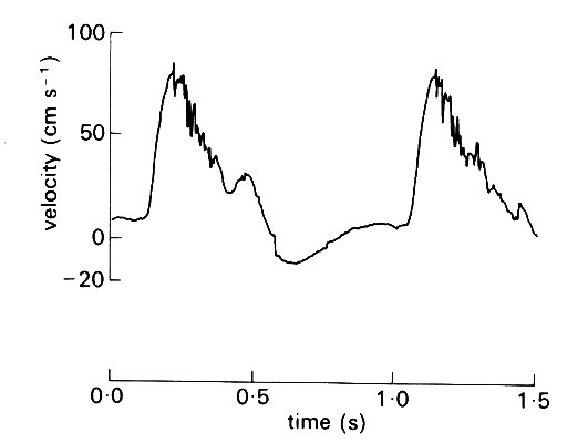
Fig. 12.49. Velocity wave-forms from the upper descending aorta of the dog, showing turbulence during the deceleration of systolic flow. (After Seed and Wood (1971). Velocity patterns in the aorta. Cardiovasc. Res. 5, 319-33.)
where high-frequency fluctuations can be seen superimposed on the underlying velocity wave-form as the flow slows down in late systole. Analysis shows that such fluctuations cover a wide frequency range, up to 500 Hz, and down to less than 25 Hz, so that they merge with the high frequency components of the main velocity wave-form. Unlike the latter, however, the velocity components at each frequency show random variation in amplitude from beat to beat, and are thus genuinely turbulent. By varying the conditions of flow (velocity and heart rate) during the experiments with drugs and nervous stimuli, it has also been shown that transition from laminar to turbulent flow does depend on both Reynolds number and a (effectively heart rate) as predicted above; this is shown in Fig. 12.50.
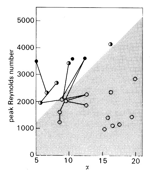
Fig. 12.50. The effect of peak Reynolds number and a on the stability of the flow in the descending aorta of anaesthetised dogs. The lines join observations made in the same animal under different conditions. Open circles: laminar flow; half-filled circles: transitional flow (disturbances only briefly seen at peak velocity); filled circles: turbulent flow. The stippled area indicates the conditions under which flow is stable and laminar. (After Nerem and Seed (1972). 'An in vivo study of aortic flow disturbances'. Cardiovasc. Res. 6, 1-14.)
However, as Fig. 12.50 shows, the aortic flow was not turbulent in the majority of experiments, and there is as yet no direct evidence about whether aortic flow is normally turbulent in the dog.
Nonetheless, there are good reasons for suspecting that it is; all the experiments shown in Fig. 12.50 were performed in animals under anaesthesia, and this strongly influences both heart rate and peak velocity of flow in a manner which would displace the points in Fig. 12.50 downwards and to the right, tending to stabilize the flow. If we examine the data which are available in the literature for normal, conscious animals (Fig. 12.51 (a)),
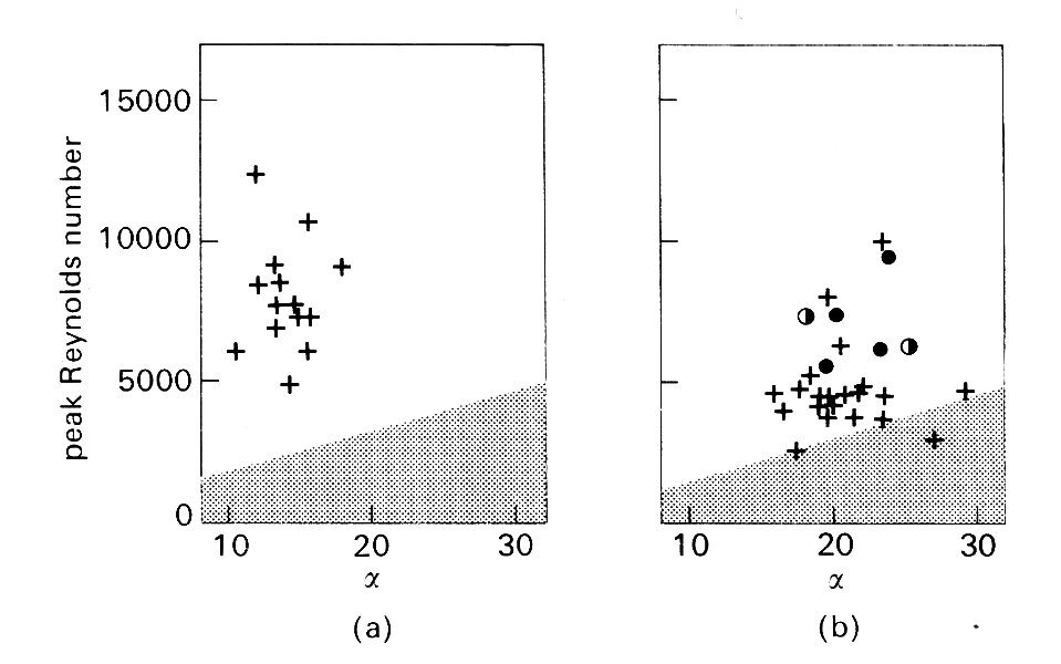
Fig. 12.51. (a) Values of peak Reynolds number and a prevailing in the ascending aorta of the normal, conscious dog. The stippled area corresponds to that in Fig. 12.50. Note that in the absence of anaesthetic effects, Re tends to be higher; all values lie in the region of the graph where turbulence would be predicted. (Data from Noble, Trenchard, and Guz (1966). Circulation Res 19, 139-47.)
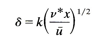
(b) Comparable data, from many sources, for normal, conscious man. Again, turbulence would be predicted in almost all cases. The circles (see caption of Fig. 12.50) show results obtained with catheter-tip hot-film probes. They demonstrate the existence of turbulence.
there are strong grounds for predicting turbulent flow. In man there are similar grounds, and also some direct evidence from studies with hot films mounted on catheters (Fig. 12.51 (b)). Thus it seems that under normal resting conditions, flow in the proximal aorta is turbulent in man and probably also in the dog. There is as yet no clear evidence about what precipitates the turbulence - upstream eddies or local disturbances in the wall-region - and little information about how far downstream it may exist.
From a fluid dynamic point of view, there is no reason why turbulence should be undesirable; the increased energy dissipation which occurs in turbulent flow would increase the pressure drop along the large arteries, but as we have seen, this is very small compared to the overall pressure drop in the systemic circulation. There are, however, a number of interesting physiological implications. The first relates to sound production. It has often been assumed that turbulence is what causes murmurs, and therefore that it is usually absent in the normal circulation; and the view that laminar flow is silent has been widely accepted. Neither of these is necessarily true. There are a number of phenomena associated with laminar flow (for example vortex shedding behind a body, §5.9) which may generate sound. There is also no a priori reason why turbulent pressure fluctuations should always be detectable at the chest wall; there might well be an audibility 'threshold'.
The presence of turbulence in a flow may have an important influence on the forces exerted by the blood on the artery wall; these may affect both the mechanical properties of the wall, and mass transfer between it and the blood (see §12.9.2). Turbulence affects these forces both through the high frequency fluctuations in pressure and shear-stress which accompany the random variations in velocity, and because the mean velocity profile and thus the mean shear-stress at the wall is altered. We first consider the mean flow. When the mean flow-rate through a straight pipe is steady, the fully-developed mean turbulent profile differs from that in Poiseuille flow, being flatter in the core, with a higher mean shear-rate at the wall (see Chapter 5). However, in the entrance region of a pipe the growing boundary-layer is thicker in turbulent flow than in laminar flow. This is because the random eddying motion causes fluid elements to be moved about laterally, so that the lateral mixing is much more effective than in laminar flow under the sole action of viscosity. The boundary-layer thickness d can still be approximately represented by an equation of the form
(see Equation (5.3), §5.3), but now the kinematic viscosity n is replaced by an effective 'eddy viscosity' n*, which incorporates the effect of turbulent mixing. One consequence of this is a shorter entry length in turbulent flow (§5.6); another is smaller mean wall shear-rates in the entrance region.
If the underlying mean* [*The word 'mean' in the context of turbulent conditions has to be defined carefully. In order to define the mean velocity we suppose that a certain flow is observed a large number of times. The measured velocity at a fixed point and a fixed time after the start of the flow will be different on each occasion because of the random turbulent fluctuations. However, if we take its average over many observations we obtain a well-defined average, called the 'ensemble average', and it is this which we call the mean velocity at that point and time. The averaging process removes all the random fluctuations, and leaves a mean which can still vary with time at any point, as, for example, when a wave passes.] flow is itself oscillatory, with angular frequency &), then the thickness of the oscillatory boundary layer will be proportional to (n/w)1/2, which is again much greater than the corresponding laminar value. Thus in flows where the laminar oscillatory boundary layer is relatively thin (a > 4) transition to turbulence will thicken it, and the mean wall shear-stress will be smaller. This conclusion applies throughout the aorta.
Another physiologically interesting implication of turbulence is in relation to the effect of vibration on the arterial wall. It is a very old clinical observation that the walls of a blood vessel often show localized dilatation just downstream of a partial obstruction to the flow, such as a narrowed (stenosed) aortic valve, for example, or an atheromatous constriction of a vessel. This post-stenotic dilatation occurs regardless of the origin of the obstruction, as long as the latter causes turbulence.
No really long-term studies have been made of the effect of vibration on arterial walls. In the short term (over periods of up to several months), however, it has been shown that post-stenotic dilatation occurs reproducibly downstream of localized stenoses (produced by partially tying off an artery) when a murmur is audible and palpable over the downstream segment. Such segments can be shown to be more distensible than normal, though there is no structural abnormality to be seen microscopically. Furthermore, excised segments of artery have been rendered more distensible by exposure to small amplitude vibrations in the frequency range 30-400 Hz for periods of several hours. This range corresponds closely to the frequency spectrum of velocity fluctuations in turbulent blood flow. Thus there is strong evidence to implicate turbulence as the cause of post-stenotic dilatation. It is interesting to speculate further that the dilatation of the aorta which takes place with age might be the result of prolonged exposure to low-amplitude vibration rather than of intrinsic degenerative changes. It has also been shown that experimentally induced turbulence may affect the permeability of the arterial wall to large molecules, and may damage the endothelium (see §12.9.2).
The main function of the circulation of the blood is to transport materials and heat to and from the tissues of the body. The exchange of material between the blood and the tissues takes place largely in the capillaries, and is therefore discussed in the next chapter. However, the walls of arteries (and veins) are also permeable, and materials are transported across them too. This transport has a nutritive function for the artery wall, but it may also play a role in the genesis of arterial disease such as atherosclerosis. In addition, it has recently been recognized that the forces exerted on the artery wall by the flowing blood may themselves be important factors in determining the permeability of the wall to large molecules, and hence may be a significant controlling influence in arterial disease. Some of this evidence is reviewed later in this section.
In order for the material which is transported to and from the tissues in the arteries and veins to be evenly distributed among the capillaries of any organ it must be well mixed in the large vessels serving that organ. The system would not function well if a stream of blood emerging from a particular organ remained as a coherent stream, unmixed with the rest of the blood, as it passed round the circulation. Furthermore a widely used method of measuring cardiac output and regional blood flow, the 'indicator-dilution technique', is also based on the assumption of good mixing between marked and unmarked blood. The extent to which mixing occurs in the heart and large vessels must therefore be examined.
12.9.1 Mixing in the heart and large blood vessels. The indicator-dilution method of measuring cardiac output was originally suggested in the nineteenth century by the physicist Adolf Fick (who also formulated the laws governing diffusion as described in Chapter 9). He pointed out that if both the difference in oxygen concentration between blood entering and leaving the lung, and the total oxygen uptake of the animal per unit time are known, then the rate of blood flow through the lung (i.e. the cardiac output) is simply the ratio of the latter to the former. Much later, when the necessary techniques of sampling and measurement had been developed, this became a standard technique for measuring cardiac output in both animals and man. So too did the derived methods of using boluses or continuous infusions of injected dye (dye-dilution), isotopically labelled materials, or thermal indicators like cooled blood or saline solution; some of these are used to measure cardiac output, others to measure the blood flow through individual organs or regions of the body. Samples of blood have to be taken at the entrance to and exit from the organ, and the concentration of indicator measured in them. It will be obvious that the method can be reliable only if the measured concentrations are actually representative of all the blood passing through the organ. For example, if the arterial blood used in the Fick calculation has an oxygen content lower than the rest of the arterial blood, the cardiac output will be overestimated.
A number of methods have been used to examine the sites, and the completeness, of mixing in the circulation. These include direct flow-visualization in transparent vessels or models following injection of coloured materials, X-ray studies of the behaviour of injected radio-opaque material within the circulation, and sampling from multiple sites after indicator injection. It is a unanimous conclusion from all these studies that an indicator passing through the heart is completely mixed with the blood by the time it emerges. On the other hand, mixing elsewhere in the circulation, or within a single chamber, may be incomplete.
Mixing in the heart appears to occur predominantly during passage of the blood through the ventricle. Samples from multiple sites in the right atrium, where streams of venous blood from different parts of the body merge, may show different concentrations of an indicator injected into a single vein, but in the right ventricle or pulmonary artery the concentration is always effectively uniform. The same conclusion holds for the left side of the heart.
The mixing which takes place in the heart is convective mixing; that is, it is a consequence of the flow patterns in the ventricle, which stir the blood and mix it up. The mixing is then much more rapid than it would be by diffusion alone, although diffusion still plays an essential part in the process as it causes the final transfer of solute from a fluid element rich in solute to an element with little, which have been brought together by the stirring. That stirring is much more effective than diffusion at mixing solute with solvent is a familiar experience, for example with a cup of tea.
It was shown in Chapter 9 that the time taken for diffusion to act over a distance Dx is proportional to tD, where
and D is the diffusivity of the material being diffused in its solvent (Equation (9.3), §9.1). Now the diffusivity of, say, oxygen in blood is about 2 x 10⁻⁹ m2s-l, so the time taken for diffusion over a distance of 1 cm (rather smaller than the distance over which diffusion would have to act in the ventricle if there were no convection) is 2 x 10⁴ s, which is far too long for complete mixing during a single heart-beat. The diffusivity of heat in blood is larger (about 10-7 m2 s-1), but still the diffusion time is too long (500 s). Only if the distance over which diffusion has to act has been reduced by convection to 0.06 cm could the mixing time for oxygen be reduced to 1 s.
In the ventricle the stirring motions of the blood are of two types. First, and probably more important, are the eddying motions set up as the blood passes through the atrioventricular valves; this has been observed in animals and in models of the left ventricle (see Chapter 11), and is a powerful mixing influence, though it does not produce complete mixing within one cardiac cycle if material is injected locally within the ventricle. The main eddy is a ring vortex around the valve-cusps; but the chordae tendinae and the irregularity of the inner walls of the ventricles must add smaller scale disturbances. These eddies will be present whether the flow is laminar or turbulent, but the second possible source of mixing is turbulence itself. We have no direct experimental evidence of turbulence in the heart, but since the Reynolds number for flow through the mitral valve may reach 8000, and since the flow into the ventricle takes the form of a jet with highly sheared edges, turbulence almost certainly does exist there for at least part of the cycle (see §5.8).
Flow in the ascending aorta is also very effective at mixing the blood, as judged from direct X-ray flow visualization and by injection of a thermal indicator into the ascending aorta. Again, the source of the stirring may lie in eddying motions either generated by the opening of the aortic valve or convected into the aorta from the ventricle (these are not necessarily turbulent), or it may arise from turbulence itself, which probably does occur in the aorta (see above).
In the descending and abdominal aorta, and the smaller arteries and veins, the evidence suggests that only partial mixing occurs. That is, samples from different sites in the vessel may have different concentrations of an indicator injected at a nearby upstream site; also continuously injected streams of radio-opaque dye remain as coherent streams. The situation here is somewhat different from that in the ascending aorta, since Reynolds numbers are lower, and turbulence does not occur. Therefore mixing can occur only through secondary motions caused by changes in geometry (bending and branching), and perhaps through the oscillatory motions, both lateral and longitudinal, which are associated with the passage of the pulse wave.
Mixing in small vessels does not appear to have been studied in the dog. In small arteries in the rabbit (0.1 cm) streaming is also seen, but in the aorta (0.3 cm) dye-streams rapidly break up and cannot be followed. In man the evidence is conflicting. It is a very old observation that dye injected into the arch of the aorta enters the two iliac arteries at different concentrations. On the other hand, injection directly into the brachial artery leads to fairly complete mixing as judged by simultaneous sampling from the radial and ulnar arteries downstream. In small veins in the rabbit, flow is largely steady, and dye-streaming suggestive of laminar flow is seen, as long as precautions like remote injection are taken to prevent the injection itself from precipitating disturbances (the presence of a needle or catheter can be a very potent source of local eddying and mixing in small vessels). In larger veins (the inferior vena cava, diameter 0.34 cm) flow is unsteady but streaming is still identifiable. In man, similar streaming can be seen radiologically in leg veins with diameters of the order of 0.5 cm, though the observation must be interpreted with caution because the appreciable density difference between blood and the radio-opaque injection medium may inhibit mixing.
There is a further interaction between flow and diffusion which influences the results of indicator-dilution studies. This is the longitudinal spreading or dispersion of a bolus of indicator as it is carried through the circulation. Some dispersion occurs because different elements of marked blood traverse pathways of different lengths within the organ being studied. However, even along a single vessel (for example, an artery) considerable dispersion is observed, far more than can be explained by pure longitudinal diffusion, with the molecular diffusivity D, as described by Equation (9.3), §9.1.
It is easiest to understand this dispersion in terms of fully developed Poiseuille flow in a long straight tube (Fig. 12.52).
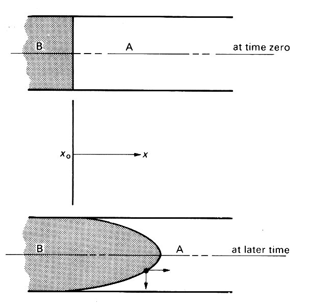
Fig. 12.52. The progressive dispersion of material B in a long tube initially full of fluid A, under Poiseuille flow conditions.
Suppose that at a certain at time zero time there is a sharp flat interface between unmarked blood A and marked blood B. As time proceeds, this interface will be pulled out into a paraboloid, the tip moving at twice the average velocity, the fluid in contact with the wall not moving at all because of the no-slip condition. If the two fluids were not able to diffuse into each other at all, there would be a progressive extension of the interface as flow proceeds.
It is possible to compute the concentration of B (averaged across a cross-section) along the tube from the origin x0 to the tip of the marked blood at x = L; the result is shown in Fig. 12.53 (broken line). However, if diffusion is possible, then a different curve is obtained because material B is capable of diffusing both axially and radially into fluid A. The axial diffusion only causes a minor blurring of the interface, but the radial diffusion is very important because it transports material B from the faster flowing core fluid to regions of lower velocity where it is transported downstream less rapidly. Consequently the longitudinal extension of the interface (dispersion) is inhibited and the concentration of B varies with distance x in a manner more like the solid curve in Fig. 12.53.
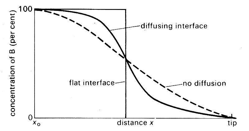
Fig. 12.53. The variation in concentration of B, averaged across a cross-section, with distance x back from the tip of the interface to its origin (x0).
The concentration profile for a flat interface is also shown. The same mechanisms operate at the rear interface if the marked blood has the form of a bolus, and the marked fluid will be distributed symmetrically about the mid-point of the bolus.
Fig. 12.53 shows how the concentration of marked fluid varies with distance at a given time. In indicator dilution studies, however, blood is sampled at a fixed position, and the concentration measured as it varies with time. It is assumed that there has been sufficient time for complete mixing across the cross-section to occur, so it is important that the measuring points are sufficiently far downstream of the injection site. As the front of the bolus arrives, the measured concentration will rise, and it will fall again at the rear. However, the graph of concentration against time will not be symmetrical about the mid-point of the bolus, whether or not parts of the bolus have traversed pathways of different lengths. The reason is that by the time the back of the bolus arrives, the mixing process has been under way for significantly longer than when the front arrived, so the tail will be more elongated than the front. It should be remembered that in physiological applications the tail of the bolus may also be strongly modified by recirculation.
In Poiseuille flow, the distribution of the bolus with distance along the pipe can be described as if there were pure diffusion, but with an effective diffusivity K which is very much larger than D.* [*This was first demonstrated mathematically by G. I. Taylor in 1953. He showed that K varies with D, with average velocity u, and with tube diameter d according to the equation
K = (ud)2/(192D) + D.
This equation has been so completely verified by experiment that it is now used as the basis of a popular method for measuring D.
If the flow is not Poiseuille flow, or if the bolus has not travelled far downstream from its origin, the above results are not quantitatively accurate. Nevertheless, the basic mechanism of dispersion caused by an axial velocity profile, and inhibited by radial diffusion, is still effective. Turbulence in the flow, or secondary motion caused by curvature or branching of the tube, stirs up the fluid and makes the lateral mixing much more vigorous than pure diffusion. This means that the axial dispersion, inhibited by lateral mixing, is significantly less than it would be in Poiseuille flow at the same flow-rate. Nevertheless it is still considerable. It has been shown, again by Taylor, that the effective longitudinal diffusion KT of any solute in fully developed turbulent flow is independent of the molecular diffusivity D. At a Reynolds number of 2300 KT takes a value of about 3.5 x 10⁻³ m2 s-1. In order to compare this with the corresponding value in Poiseuille flow (K) we must consider a particular case, for example the dispersion of oxygen in blood, where D = 2 x l0-9 m2 s-1. When Re =2300, the value of K is about 250, and the turbulent value is smaller by a factor of about 10-5; nevertheless it is still two million times greater than the molecular value D. A bolus of dissolved oxygen in an artery at this value of the Reynolds number will spread out to occupy a length (2Kt)1/2 in time t (Equation (9.3), §9.1, with D replaced by K). If the flow is turbulent and t = 1 s, this is a length of 8 cm; if Poiseuille flow is present, it is a length of 20 m; if the flow is laminar, but disturbed by secondary motions, we do not know what the length is, although it will lie between the two and we expect it to be closer to the turbulent value because the mechanism of lateral mixing is similar. It is appropriate to mention here that it has been predicted that the effective diffusivity can be increased even above the Poiseuille flow value if longitudinal pulsations are imposed on the flow; this prediction has not yet been confirmed experimentally.12.9.2 Mass transport across artery walls. The artery wall is metabolically active, so that materials have to be transported to and from it. One route for this transport is through the vasa vasorum, which arise from both adventitial arteries and from the vessel lumen, and appear to supply the adventitia and the media of large arteries (§12.1.3). However, the intima of systemic arteries is devoid of capillaries, and appears to be supplied across the endothelium, which is the other major route for mass transport. These conclusions are based on studies of uptake of labelled materials from the blood into the artery wall in vivo. Transport by the vasa vasorum has not been extensively studied because of technical difficulty, and we consider it no further. However, the trans-endothelial route has recently been the subject of numerous studies, because among other reasons it is believed to be implicated in the development of atheroma.
Atheroma nowadays increasingly manifests itself as a disease process in middle rather than old age; however, changes in the large arteries are apparent at postmortem even in young subjects, and many people believe that these are the early stages of atheroma. The earliest change visible under the microscope is the accumulation of lipid in the tunica intima, in so-called fatty streaks, which are covered by an intact layer of endothelium and do not deform the vessel wall. At a subsequent stage, raised plaques become visible on the internal surface of the artery. The endothelium overlying these may still be intact, and their microscopic structure is quite variable, depending upon the relative proportions of free fat deposits, fat-laden ('foam') cells, and fibrous (scar) tissue. Later, the endothelium may break down, bringing these elements into direct contact with the blood. The endothelium may then regrow, or the plaque may increase in size due to further fat deposition and scarring and the progressive accumulation of layers of thrombus (formed through aggregation of platelets, by the mechanism described in Chapter 10). This thrombus may remain in situ, gradually being destroyed by cells which infiltrate it, and covered by a layer of endothelium which grows over it; even if the vessel is completely blocked, it frequently recanalizes in this way. Alternatively, pieces of thrombus may be shed into the vessel to lodge in a smaller branch downstream. Such fragments are known as emboli, and cause a variable amount of damage depending upon the downstream anatomy, particularly the extent of interconnections—anastomoses—between the small vessels which can by-pass the block. Interruption of the blood supply to vital organs by atheromatous lesions or their complications is nowadays responsible for about half the deaths that occur in most developed countries. The chief sites are the brain ('stroke') and heart (myocardial infarction).
Atheroma occurs patchily, developing preferentially at certain sites in the cardiovascular system. For example, both early atheromatous plaques and fatty streaks are generally found in the major central arteries and not in the peripheral circulation.* [*We concentrate here on early manifestations of atheroma, because advanced lesions may themselves have a significant influence on the blood flow past them, and hence on the development of atheroma at neighbouring sites.] Within an artery early atheroma is more often to be found near junctions than elsewhere; the abdominal aorta is more severely affected than the thoracic aorta; the posterior wall of the descending thoracic aorta almost always exhibits fatty streaking while the anterior wall does not; the carotid sinus is usually severely affected. Such a preferential distribution of atheroma can arise in one or both of two ways: either the normal structure of artery walls varies, so that some areas are predisposed to develop atheroma, or they are subjected to different influences (for example, different shear-stresses exerted by the blood) so that some physiological or biochemical process is altered. The first possibility is currently being investigated, but so far the second alternative has generally been preferred.
The fatty streaks observed in arteries represent an accumulation of lipid, much of which is in the form of cholesterol esters, in the tunica intima. Lipid deposition is also observed in early atheromatous plaques, together with other changes including accumulation of protein and some thickening of the fibrous and muscular layers. Some of this lipid is thought to be transported to the site from the blood and 'deposited' there, a process which presumably represents a slight net imbalance between the fat transported into the wall and that which simultaneously is degraded or transported out; mass transport is of course a two-way process, and a state of equilibrium requires a balance between incoming and outgoing molecules of the material. But other lipid is contained within cells, and is believed to be manufactured there. In this case a net accumulation of lipid would require that it be more difficult for the fat to escape from the wall and into the blood than for its precursors (whatever they are) to be transported in. As well as small molecules, these precursors probably include plasma lipoproteins, since cholesterol is not soluble in plasma, and must therefore be transported in conjunction with a protein that is. The observations briefly summarized above have led to the hypothesis that atheroma develops in regions of the artery wall where for some reason the rate of efflux of lipids or lipoproteins from the wall is slightly inhibited relative to other wall regions. Support for this hypothesis comes from experiments in which animals are fed high cholesterol diets. In these animals the blood cholesterol level is much higher than normal, and fatty streaks develop preferentially in those regions of the wall which, from human postmortem studies, we would expect not to be affected. This suggests that influx of cholesterol from the blood to the wall, driven by a concentration difference assumed to be the reverse of normal, is enhanced in just those regions where, normally, there are no fatty streaks. (At a later stage in such studies lipid is found to accumulate in the same regions as in man.) The above hypothesis has led to a number of in vitro and in vivo experiments designed to examine the permeability of arterial endothelium to proteins, or lipoproteins and other large molecules, and to investigate the effect of haemodynamic forces on the permeability.
Many such experiments have been performed in vivo with the dye Evans Blue, which is bound to albumin in the plasma. Regions in which the rate of albumin transport into the wall is relatively large show up after postmortem dissection because they are stained blue. A blue-stained area is one which is relatively permeable to albumin; the flux of marked albumin is proportional to the concentration gradient of marked albumin, and is independent of any other albumin which may be present. The unmarked albumin remains in dynamic balance as it was before injection of the marked albumin; presumably the rate at which unmarked albumin passes into and out of the wall is also increased in blue-stained areas, but this does not affect the equilibrium levels. No inference can be made from Evans Blue experiments about the total amount of albumin in the wall. The permeability can be deduced because in sufficiently short-term studies it is proportional to the rate at which the concentration of unmarked albumin in the wall increases.
The obvious implication that a piece of artery with an enhanced permeability to albumin also has an enhanced permeability to other proteins and lipoproteins has been borne out by studies with radioactively marked fibrinogen and cholesterol, the latter presumably bound to a protein. All these studies have indicated that endothelial permeability is greater in those regions of the wall which are normally spared from early atheroma, but which in cholesterol-fed animals initially exhibit lesions. Thus the hypothesis that early atheroma is normally associated with low permeability of the endothelium, inhibiting the efflux of cholesterol, is borne out. The question now arises as to what controls the permeability of the endothelium.
One of the most popular suggestions is that the differences in the forces exerted on the wall by the flowing blood are responsible for the differences in permeability. These forces consist of the pressure and the viscous shearing stress. At any point of the artery wall both these quantities have well denned mean values, about which they oscillate every time the pulse wave passes, and they may also include random high-frequency components if there is turbulence present.
One of the first suggestions was that atheroma is associated with damage to the endothelium caused by high wall shear-stresses, since it was shown that a shear-stress greater than 40 N m~2 can damage endothelial cells. However, as we show below, the shear-stress in blood vessels is normally considerably smaller than this, and it would require the local geometry of the vessel wall to be already distorted for such high stresses to arise. In any case, it has subsequently been demonstrated in vitro that the main effect of damaging the endothelium is to increase its permeability to large molecules, which according to the above ideas would not be expected to lead to atheroma.
A more recent hypothesis has been that atheroma develops most readily in regions where the mean wall shear-stress is relatively low. This was based on both the observed distribution of fatty streaks in human arteries, and also fluid dynamical predictions of regions where the mean shear-stress is low. The observations on fatty streaks included those referred to above, showing that, except along the aorta, fatty streaking develops less readily at more peripheral sites. Also included were data on the local distribution of fatty streaking near junctions (the outer walls of the junction, Fig. 12.44, were seen to be affected, but the flow divider tended to be spared) and in curved arteries (more fatty streaking on the inside of the bend) and in the carotid sinus. The regions which tend to be spared from fatty streaking are those which are normally found to be more permeable to large molecules.
The fluid dynamic predictions were based on the known distribution of shear-stress in tubes when the flow is steady, on the assumption that the mean flow in pulsatile conditions is similar to steady flow with the same average velocity. The shear-stress on the wall in Poiseuille flow, with an average velocity equal to u, is
t0 = 8m u/d (12.29)
where m is the viscosity of the blood, and d the tube diameter (see §5.1). If Poiseuille flow were present in all blood vessels then the wall shear-stress would be distributed along them as shown in Table 12.3, constructed from the data on dog's vessels given in Table I. This shows a marked increase (about tenfold) from the aorta to the arterioles, and supports the contention that the lack of fatty streaking in small arteries is related to a greater mean shear-stress there. Of course, the mean flow within an artery is not Poiseuille flow, because there is an entrance length (so that the mean shear in the ascending aorta is much larger than that shown in Table 12.3, consistent with the finding of greater permeability there), and there are secondary motions caused by bends and branches. Greater fatty streaking on the inside of a bend is consistent with the lower shear-stress to be expected there (§12.8.2). Again, the details of steady flow in junctions (§12.8.2) shows that the shear-stress would indeed be high on the flow divider and low on the outer walls, consistent with the observations of fatty streaking.* [*This is not as clear-cut as it appears, however, because model experiments on flow through a cast of the aorta have shown that the distribution of shear-stress near junctions (for example, of the coeliac and mesenteric arteries) is very sensitively dependent on the precise local geometry. If the far lip of a junction (the flow divider in Fig. 12.47) protrudes by 0.5 mm into the lumen of the aorta, the shear-stress just beyond it is reduced, not enhanced, presumably because of flow separation.]
Table 12.3. Wall shear-stress (Nm-2)
|
|
| Ascending aorta | 0.43 |
| Abdominal aorta | 0.53 |
| Femoral artery | 0.80 |
| Arteriole | 4.8 |
| Capillary | 3.7 |
| Venule | 3.0 |
| Inferior vena cava | 0.64 |
|
Main pulmonary artery |
0.28 |
The 'low mean shear-stress' hypothesis is thus a very attractive one. However, it does involve the assumptions that the unsteady components of the shear-stress have no qualitative effect on the distribution of permeability, and that the mean shear-stress in unsteady flow is distributed in a similar way as the shear-stress in steady flow. The second assumption may be approximately justified (because the oscillatory part of the flow is fully developed except very the shear-stress just beyond it is reduced, not enhanced, presumably because of flow separation. near the entrance of a tube, and can be shown theoretically not to affect the mean) but the first is less easy to justify. This is because the unsteady shear-stresses in arteries are expected to be extremely large compared with the mean shear-stress. To illustrate this, we consider fully developed sinusoidal flow in a straight pipe, with mean velocity u, velocity amplitude u1, and a large value of the frequency parameter a. The mean wall shear-stress is t0 (Equation (12.29)), and the amplitude of the shear-stress oscillations is 2am u1/d. We can apply these results to flow in the human aorta, where d is about 2.5 cm, u is about 0.2 m s-1, and u1 about 1 m s-1. Using a value of a of 20, we see that the peak oscillatory shear-stress is approximately 6.4 N m-2, which is some 25 times the mean. Furthermore, when the composite velocity wave-form contains higher frequency oscillations (as occurs in vivo) the shear-stress amplitude becomes larger still (up to 50 times the mean). It seems unlikely that the permeability of endothelial cells should depend on the low mean shear-stress, when the level of shear-stress actually experienced is so much greater.
Thus the 'low mean shear-stress' hypothesis cannot be established until the mechanism by which shear-stress controls endothelial permeability is understood, and as yet it is not. A number of experiments on perfused excised segments of artery have been carried out, and the uptake of radioactively marked substances measured quantitatively in various flow situations. Several possible mechanisms have been eliminated in this way, but the real one is yet to be discovered.
One suggestion was that the permeability is dictated by the ease with which large molecules travel through the channels between endothelial cells, by diffusion or filtration. However, there is no direct evidence of large molecules (m.w. greater than 70,000) taking this path.
Another suggestion was that the rate of transport into the wall is controlled by a thin mass transfer boundary-layer (Chapter 9, §9.9) across which the concentration of solute varies from its value in the core of the artery to its value at the wall. This mechanism has the virtues that it would be shear-dependent, and that it can be clearly demonstrated that it is the mean shear which is important, not the fluctuations. However, the quantitative in vitro studies have shown that the resistance to mass transport into the wall is about 1000 times greater than could possibly result from a boundary-layer in the blood. Furthermore, the longitudinal variation of uptake along an excised segment of artery, predicted because the mass transfer boundary layer would grow with distance along it (Equation (9.19) or (9.22)), was entirely absent.
Thus the resistance to transport of large molecules across the endothelinm must lie in the cells themselves. Possible mechanisms of transport include so-called 'pinocytosis', in which small vesicles at the cell surface entrap small amounts of plasma, carry them bodily across the cell, and release them into the intima. Such a process might be a passive, diffusional one, or it might involve active mechanisms. Other types of active transport might also be involved. No mechanism of this type has yet been proposed which would show how shear-stress could affect permeability, although the observation has been made in vitro that an effectively steady shear-stress does enhance the permeability to macromolecules. There is also some evidence that the presence of turbulence not only affects the elastic properties of the artery wall (§12.8.3) but also makes the endothelium more permeable. This could be part of the explanation of greater permeability variations observed in the neighbourhood of junctions where flow separation and therefore turbulence might occur.
Because of their value as an aid to the interpretation of physiological measurements, the mathematical forms of the relationships referred to in the text are widely used by physiologists. We therefore quote them here, although they require the use of complex numbers which we have elsewhere tried to avoid. In these terms, the equation for the pressure in a wave travelling in the positive x-direction (cf. Equation (12.20)) is
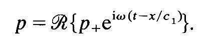 (12.30)
Here i = (-l)1/2, e is the familiar exponential function, which has the property that
eiz = cos z + i sin z
and the symbol R means that the real part of the complex quantity on the right-hand side has to be taken. Thus if p+ is itself a complex number of the form
p+ = pa + i pb
Equation (12.30) means
p = pa cos {w(t-x/c1)} - pb sin {w(t-x/c1)}.
Similar expressions can be written for the flow-rate and for waves travelling in the opposite direction. It is conventional to omit the symbol R, so that whenever a complex number is supposed to represent a physical quantity, it is assumed that its real part is being used.
With complex numbers it is possible to write down the ratio of the pressure and flow-rate at a point, for example the point A in a tube AB (Fig. 12.28), by means of a complex quantity called the effective impedance, Z1 eff:
![]() (12.31)
(12.31)
Calculations for the double junction in Fig. 12.28 shows that Z1 eff can be expressed in terms of the characteristic impedance of the tube AB, Z1 (= rc1/A1 where A1, c1 are the area and wave-speed of that tube) and of the effective impedance of tubes 3 and 4 at B. The result is
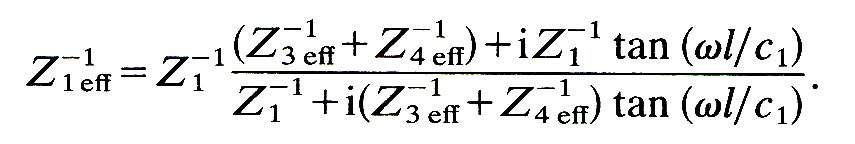 (12.32)
By repeated use of this equation, it is possible, as described above, to relate the excess pressure and flow-rate in the parent tube of a complicated network, given their values at the distal end. It must be remembered that Equation (12.31) refers just to waves of a single frequency w. In order to relate the pressure and flow-rate of a composite wave with many frequency components, the calculation must be repeated for each one. The effective impedance at A, Z1 eff, is often called the input impedance of the system distal to A.
We may note the dependence of Equation (12.32) on the ratio between the length l of AB and the quantity c1/w (equal to l/2p times the wavelength of the wave in AB). If wl/c1 is very small, then so is tan (wl/c1), and
Z1 eff-1 = Z3 eff-1 + Z4 eff-1
That is, if l is much smaller than the wavelength, the tube AB forms part of the junction, and its properties are irrelevant. A similar result holds if wl/c1 is equal to a whole number of multiples of p, i.e. if l is equal to a whole number of half-wavelengths, as predicted above. However, if wl/c1 is equal to an odd multiple of p/2 (l equal to an odd number of quarter-wavelengths), tan (wl/c1) is infinite, and
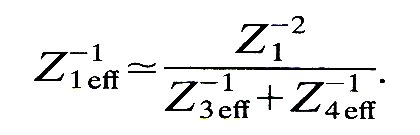
In this case, if Z1-1 is less than Z3 eff-1 + Z4 eff-1, Z1 eff-1 is smaller still, and vice versa. This agrees with the earlier conclusion (§12.4.5) that the wave eventually transmitted will be large if the reflection at B is positive (Z1-1 > Z3 eff-1 + Z4 eff-1), and small if it is negative.
The effective, or input, impedance of a system is a complex number, so it has real and imaginary parts Zr and Zi:
Zeff = Zr + i Zi
In many analyses of the cardiovascular system this is re-written in the following, rather different, form:
Zeff = M eiq (12.33)
Here M is the magnitude, or modulus, of the impedance, given by
M = (Zr + Zi)1/2
and q is its phase, given by
tan q = Zi/Zr
The modulus, M, represents the magnitude of the opposition to flow offered by the system distal to the point of measurement, and q represents the phase lead of pressure over flow-rate. The dependence of these quantities on more distal conditions can be seen, by using Equation (12.32) in conjunction with Equation (12.33), to be very complicated.
The idea of impedance is very useful both for predicting the relationship between the pressure and flow-rate wave-forms in a system, and for interpreting data. However, it is also a concept which has caused considerable confusion among physiologists because of the temptation to use the word without being very clear about its meaning. Part of the trouble lies in the large number of slightly different quantities all called impedance. We list many of them here, not because we recommend their use but rather in the hope that familiarity with them all will help to avoid confusion. We have already met the characteristic impedance Z of a tube: the ratio of pressure to flow-rate in that tube when a sinusoidal wave is travelling along it at constant speed in one direction. For elastic tubes containing non-viscous fluid, which we have taken as models of arteries so far, this is a real quantity, indicating that the pressure and flow-rate wave-forms are in phase. A related quantity is the longitudinal impedance ZL, which is the ratio of pressure gradient to flow-rate when the same type of wave is propagating (it therefore has different dimensions from other impedances: [ML-5T-1] not [ML-4T-1]). In the tubes considered so far this is a purely imaginary quantity (ZL = -iwZ/c), since the pressure gradient and flow-rate are 90° out of phase. In a straight rigid tube in which the frequency is so low that Poiseuille flow is always present, the pressure gradient and flow-rate are in phase, so ZL is real, and Z is imaginary. Another quantity we have already met is the effective impedance Zeff of a system, equal to the ratio of pressure and flow at the entrance to the system. This is also called input impedance, especially when it refers to the whole vascular bed, and sometimes even terminal impedance, when it refers to that part of the vascular bed distal to the part of current interest. Finally there is the term source impedance, which refers to a flow source or pump, e.g. the heart. If a pump is short-circuited, so that the flow from its output is pumped directly into its input, the system to which it is connected has negligible impedance. Nevertheless, any real pump will produce only a finite flow-rate, Q, and there will be a non-zero pressure difference Dp across it. Their ratio, Dp/Q, is therefore not zero, and the circuit as a whole has non-zero impedance, which is all associated with conditions in the pump itself. This 'source impedance' is present whatever system the pump is pumping into.
The source impedance of the left ventricle, at any volume, is thus equal to the difference between the maximum pressure which the muscles could exert at that volume (under isometric contraction) and the actual ventricular pressure, divided by the volume flow-rate out of the heart. In early systole, this quantity is about six times the input impedance of the aorta, indicating that the normal myocardium contracts as rapidly as allowed by its own rate-limiting mechanisms (represented by the force-velocity relationship, see Chapter 11) rather than by the load it pumps against. Later in systole, however, the source impedance falls, and the aortic load increases in importance.
BERGEL, D. H. (1972) (ed.). Cardiovascular fluid dynamics. Chapter 2: 'Pressure measurement in experimental physiology', by I. T. Gabe; Chapter 3: 'Measurement of pulsatile flow and flow velocity', by C. J. Mills; Chapter 9: 'Pressure and flow in large arteries', by D. L. Schultz; Chapter 10: 'Vascular input impedance', by U. Gessner; Chapter 11: 'The rheology of large blood vessels', by D. J. Patel and R. N. Vaishnav; Chapter 12: 'The influence of vascular muscle on the viscoelastic properties of blood vessels', by B. S. Gow; Chapter 13: 'Post-stenotic dilatation in arteries', by M. R. Roach; Chapter 19; 'Synthesis of a complete circulation', by R. Skalak. Academic Press, London and New York. (2 vols)
BERGEL, D. H. and SCHULTZ, D. L. (1971). Arterial elasticity and fluid dynamics. Prog. Biophys. Molec. Biol. 22 (ed. J. A. V. Butler and D. Noble).
CHARM, S. E. and KURLAND, G. S. (1974). Blood flow and microcirculation. John Wiley, New York.
CIBA FOUNDATION SYMPOSIUM (1969). Circulatory and Respiratory Mass Transport. Articles on: 'The optimum elastic properties of arteries', and 'Velocity distribution and transition in the arterial system', J. & A. Churchill Ltd., London.
CIBA FOUNDATION SYMPOSIUM (1973). New Series, No. 12. Atherogenesis: Initiating Factors. Associated Scientific Publishers, Amsterdam.
FUNG, Y. C., PERRONE, N., and ANLIKER, M. (1972) (ed.). Biomechanics: Its foundations and objectives. Chapter 5: 'The properties of blood vessels', by D. H. Bergel; Chapter 15: 'Toward a non-traumatic study of the circulatory system', by M. Aniiker; Chapter 16: 'Flow and pressure in the arteries', byT. Kenner. Prentice-Hall, New Jersey.
GUYTON, A. C. and JONES, C. E. (1974) (ed.). Cardiovascular physiology. Chapter 1: 'The mechanics of the circulation', by C. G. Caro, T. J. Pedley, and W. A. Seed. M.T.P. International Review of Science. Butterworth & Co. Ltd., London, and University Park Press, Baltimore.
LIGHTHILL, M. J. (1975). Mathematical biofluid dynamics. S.I.A.M., Philadelphia.
MCDONALD, D. A. (1968). Haemodynamics. A. Rev. Physiol. 30, 525-56.
MCDONALD, D. A. (1974). Blood flow in arteries (2nd ed.). Edward Arnold, London.
PATEL, D. J., VAISHNAV, R. N., Gow, B. S., and KOT, P. A. (1974). Haemodynamics. A Rev. Physiol. 36, 125-54.
TAYLOR, M. G. (1973). Haemodynamics. A. Rev. Physiol. 35, 87-116.
WHITMORE, R. L. (1968). Rheology of the circulation. Pergamon Press, Oxford.